S1 CSE Maths · Module 1

Page 1 of 19

Module 1 at a glance

This module teaches one big idea in three steps: limits → derivatives → using derivatives.

Limits tell us what value a function is going towards near a point, even if it never reaches that point.
Derivatives are a special kind of limit. They tell us how fast a function is changing. This is the same as the slope of its graph.
Applications use derivatives for real work: tangent and normal lines, straight-line approximation (linearization) and the bending of a curve (concavity).

What you will be able to do

Find limits by substitution, factorising, rationalising, the sandwich theorem, and "divide by the highest power".
Check whether a function is continuous at a point, and find where it is not.
Differentiate from first principle and with the standard rules, including the chain rule and implicit differentiation.
Write the equation of a tangent line and a normal line.
Find an approximate value of a function near a point using linearization.
Use the second derivative to find where a curve bends up or down.

How to use these notes

Every topic has the same shape: idea → rule → worked example → common mistakes.
Try each worked example yourself first. Cover the answer, solve it, and then compare.
Green boxes hold key ideas. Amber boxes marked Watch out show the mistakes that make you lose marks.
The last page is a one-page formula sheet. Use it for revision before the exam.

Where each topic sits

Part	Topics
Limits	Limits, limit laws, techniques for $0/0$ , sandwich theorem, limits at infinity
Continuity	Continuity at a point, one-sided limits, where a function breaks
Derivatives	First principle, rules, higher orders, rate of change, chain rule, implicit differentiation
Applications	Tangent and normal lines, linearization, concavity

Before you start. You should know how to factorise quadratics, the formula $(a-b)(a+b)=a^2-b^2$ , laws of indices (e.g. $x^{-2}=1/x^2$ , $\sqrt{x}=x^{1/2}$ ), and the values of $\sin$ , $\cos$ , $\tan$ at $0,\ \pi/6,\ \pi/4,\ \pi/2$ .

Page 2 of 19

Limits of function values

The idea

A limit answers this question: "As $x$ gets very close to $c$ , what value is $f(x)$ getting close to?"

If $f(x)$ comes as close as we like to a number $L$ when $x$ is close enough to $c$ (but $x \ne c$ ), we write

\lim_{x \to c} f(x) = L

and say " $f$ approaches $L$ as $x$ approaches $c$ ".

Key idea. A limit is about what happens near $c$ , not at $c$ . The function need not even be defined at $c$ . That is why limits help us when substitution gives the meaningless $0/0$ .

Example: a hole in the graph

Find $\displaystyle\lim_{x\to 1}\frac{x^2-1}{x-1}$ .

If we put $x=1$ , we get $0/0$ , so the function is not defined at $1$ . For $x\ne1$ we can cancel the common factor:

\frac{x^2-1}{x-1}=\frac{(x+1)(x-1)}{x-1}=x+1 \qquad (x\neq 1)

So near $x=1$ the function behaves exactly like $x+1$ , and

\lim_{x\to1}\frac{x^2-1}{x-1}=1+1=\mathbf{2}

The graph is the line $y=x+1$ with one hole at $(1,2)$ . The limit is the height of that hole.

Two simple limits to remember

Identity function $f(x)=x$ : as $x\to c$ , the output is $x$ itself, so

\lim_{x\to c} x = c

{
  "boundingBox": [-1, 5, 5, -1],
  "axis": true,
  "points": [],
  "segments": [],
  "circles": [],
  "functions": [{ "expression": "x", "label": "f(x): y = x" }]
}

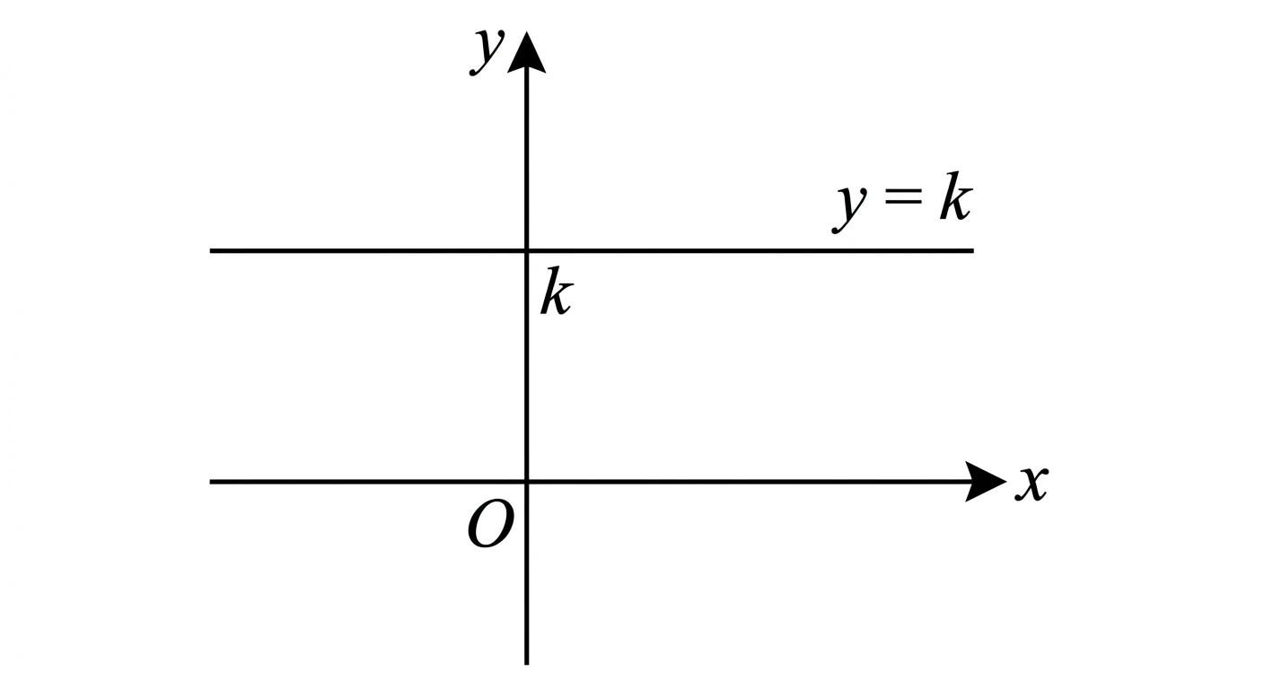
Constant function $f(x)=k$ : the output never changes, so

\lim_{x\to c} k = k

Graph of the constant function y = k, a horizontal line at height k

When a limit does not exist

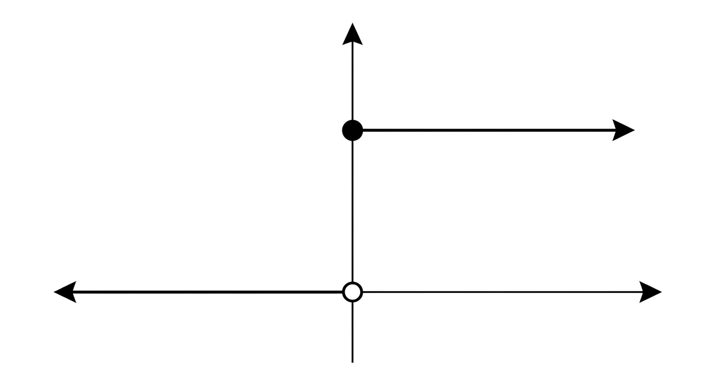
Consider the unit step function

u(x)=\begin{cases}0, & x<0\\[2pt] 1, & x\ge 0\end{cases}

Graph of the unit step function u(x): 0 to the left of the y-axis, jumping to 1 at x = 0

When $x$ comes to $0$ from the left ( $x<0$ ), $u(x)$ stays at $0$ .
When $x$ comes to $0$ from the right ( $x>0$ ), $u(x)$ stays at $1$ .

There is no single number that $u(x)$ goes to, so $\displaystyle\lim_{x\to0}u(x)$ does not exist. The graph jumps.

Rule of thumb. A limit exists only when the function goes to the same value from both sides.

Page 3 of 19

Limit laws

Suppose $\lim_{x\to c}f(x)=L$ and $\lim_{x\to c}g(x)=M$ , where $L$ , $M$ , $c$ , $k$ are real numbers. Then:

Rule	Statement
Sum	$\lim\,[f(x)+g(x)] = L+M$
Difference	$\lim\,[f(x)-g(x)] = L-M$
Constant multiple	$\lim\,[k\,f(x)] = kL$
Product	$\lim\,[f(x)\,g(x)] = L\cdot M$
Quotient	$\lim\,\dfrac{f(x)}{g(x)} = \dfrac{L}{M}$ , provided $M\neq0$
Power	$\lim\,[f(x)]^n = L^n$
Root	$\lim\,\sqrt[n]{f(x)} = \sqrt[n]{L}$ (for even $n$ , need $L\ge0$ )

In simple words: you can take the limit inside $+,\ -,\ \times,\ \div$ , powers and roots, as long as each part has its own limit (and you never divide by a limit equal to $0$ ).

Watch out. The root and power rules work on the whole expression inside. The root of a sum is not the sum of the roots: $\sqrt{16+3}\neq\sqrt{16}+\sqrt{3}$ . First find the limit of what is inside, then take the root.

Polynomials and rational functions: just put the value

If $P(x)=a_nx^n+\dots+a_1x+a_0$ is a polynomial, then

\lim_{x\to c}P(x)=P(c)

If $f(x)=\dfrac{P(x)}{Q(x)}$ is a rational function, then

\lim_{x\to c}\frac{P(x)}{Q(x)}=\frac{P(c)}{Q(c)}\qquad\text{provided } Q(c)\neq0

Example 1. Substitution works

\lim_{x\to c}(x^3+4x^2-3)=c^3+4c^2-3

\lim_{x\to-1}\frac{x^3+4x^2-3}{x^2+5}=\frac{(-1)+4-3}{1+5}=\frac{0}{6}=\mathbf{0}

Example 2. Root of an expression

\lim_{x\to2}\sqrt{4x^2+3}=\sqrt{4(2)^2+3}=\sqrt{16+3}=\mathbf{\sqrt{19}}

Example 3. Substitution fails (the $0/0$ case)

\lim_{x\to1}\frac{x^2+x-2}{x^2-x}\ \longrightarrow\ \frac{1+1-2}{1-1}=\frac{0}{0}

$\tfrac00$ is not the answer. It is a signal that the top and the bottom have a hidden common factor. Factorise, cancel, and then substitute:

\frac{x^2+x-2}{x^2-x}=\frac{(x+2)(x-1)}{x(x-1)}=\frac{x+2}{x}\ \Rightarrow\ \lim_{x\to1}\frac{x+2}{x}=\frac{3}{1}=\mathbf{3}

The next page gives a method for this.

Page 4 of 19

Finding limits: a method with the same first step every time

Step 0: try substitution

Put $x=c$ in the expression.

If you get a number, that number is the limit. Done.
If you get $k/0$ with $k\neq 0$ (for example $5/0$ ), the function becomes very large. The limit does not exist (as a finite number).
If you get $0/0$ , this is an indeterminate form. The limit may still exist. Use one of the techniques below.

Technique A: factorise and cancel

Use this when the expression is a ratio of polynomials.

Quick factorising tip. To factorise $x^2+bx+c$ , find two numbers whose product is $c$ and whose sum is $b$ . For $x^2-6x+9$ : product $9$ , sum $-6$ → $(x-3)(x-3)$ .

Example. $\displaystyle\lim_{x\to-5}\frac{x^2+3x-10}{x+5}$

Substitution gives $0/0$ . Product $-10$ , sum $3$ , so the numbers are $5$ and $-2$ :

\frac{x^2+3x-10}{x+5}=\frac{(x+5)(x-2)}{x+5}=x-2\ \Rightarrow\ \lim_{x\to-5}(x-2)=\mathbf{-7}

Technique B: multiply by the conjugate

Use this when there is a square root in the numerator or denominator. The conjugate of $\sqrt{A}-B$ is $\sqrt{A}+B$ , and

(\sqrt{A}-B)(\sqrt{A}+B)=A-B^2

which removes the root. Multiply the top and the bottom by the conjugate, so the value of the fraction does not change.

Example. $\displaystyle\lim_{x\to0}\frac{\sqrt{x^2+100}-10}{x^2}$

\begin{aligned} &=\lim_{x\to0}\frac{(\sqrt{x^2+100}-10)(\sqrt{x^2+100}+10)}{x^2\,(\sqrt{x^2+100}+10)}\\[4pt] &=\lim_{x\to0}\frac{(x^2+100)-100}{x^2\,(\sqrt{x^2+100}+10)}\\[4pt] &=\lim_{x\to0}\frac{x^2}{x^2\,(\sqrt{x^2+100}+10)}=\lim_{x\to0}\frac{1}{\sqrt{x^2+100}+10}\\[4pt] &=\frac{1}{10+10}=\mathbf{\tfrac1{20}} \end{aligned}

Technique C: simplify a fraction inside a fraction

Example. $\displaystyle\lim_{x\to1}\frac{x^{-1}-1}{x-1}$ . Substitution gives $0/0$ .

\frac{\tfrac1x-1}{x-1}=\frac{\tfrac{1-x}{x}}{x-1}=\frac{-(x-1)}{x\,(x-1)}=-\frac1x \ \Rightarrow\ \lim_{x\to1}\left(-\frac1x\right)=\mathbf{-1}

Watch out. Cancel only factors, never terms. In $\dfrac{x+3}{x}$ you cannot cancel the $x$ 's. You can cancel $(x-c)$ because $x\to c$ means $x\neq c$ , so $x-c\neq0$ .

Page 5 of 19

Solved limit problems

The problems are grouped by the technique used. Try each one before looking at the answer.

Group 1: direct substitution

#	Limit	Working	Answer
1	$\lim_{x\to-2}(x^3-15)$	$(-2)^3-15=-8-15$	$-23$
2	$\lim_{x\to2}(-x^2+5x-2)$	$-4+10-2$	$4$
3	$\lim_{x\to2}\dfrac{2x+5}{11-x^3}$	$\dfrac{9}{11-8}=\dfrac93$	$3$
4	$\lim_{x\to\frac23}(8-3x)(2x-1)$	$(8-2)\left(\tfrac43-1\right)=6\cdot\tfrac13$	$2$
5	$\lim_{x\to-\frac12}4x(3x+4)^2$	$-2\cdot\left(\tfrac52\right)^2=-2\cdot\tfrac{25}{4}$	$-\tfrac{25}{2}$
6	$\lim_{y\to-3}(5-y)^{4/3}$	$8^{4/3}=(2^3)^{4/3}=2^4$	$16$
7	$\lim_{h\to0}\dfrac{3}{\sqrt{3h+1}+1}$	$\dfrac{3}{1+1}$	$\tfrac32$
8	$\lim_{h\to1}\dfrac{\sqrt{6h+10}-5}{h^2}$	$\dfrac{4-5}{1}$	$-1$
9	$\lim_{x\to3}\dfrac{x+4}{x^2+7x+14}$	$\dfrac{7}{9+21+14}$	$\tfrac{7}{44}$
10	$\lim_{t\to2}\dfrac{t^2+4t+3}{t^2-9}$	$\dfrac{4+8+3}{4-9}=\dfrac{15}{-5}$	$-3$
11	$\lim_{x\to0}(2\sin x-1)$	$2\sin0-1$	$-1$
12	$\lim_{x\to0}\dfrac{1+x+\sin x}{2\cos x}$	$\dfrac{1+0+0}{2\cdot1}$	$\tfrac12$
13	$\lim_{x\to\pi}\sqrt{x+2}\,\sin\dfrac x2$	$\sqrt{\pi+2}\cdot\sin\tfrac\pi2$	$\sqrt{\pi+2}$

Group 2: $0/0$ , so factorise

14. $\displaystyle\lim_{x\to3}\frac{x^2-6x+9}{x-3}=\lim_{x\to3}\frac{(x-3)^2}{x-3}=\lim_{x\to3}(x-3)=\mathbf{0}$

15. $\displaystyle\lim_{x\to-4}\frac{2x+8}{x^2+x-12}=\lim_{x\to-4}\frac{2(x+4)}{(x+4)(x-3)}=\frac{2}{-4-3}=\mathbf{-\tfrac27}$

16. $\displaystyle\lim_{x\to5}\frac{x-5}{x^2-25}=\lim_{x\to5}\frac{x-5}{(x+5)(x-5)}=\frac1{10}$

17. $\displaystyle\lim_{x\to2}\frac{x^2-7x+10}{x-2}=\lim_{x\to2}\frac{(x-5)(x-2)}{x-2}=2-5=\mathbf{-3}$

18. $\displaystyle\lim_{t\to-2}\frac{-2t-4}{t^3+2t^2}=\lim_{t\to-2}\frac{-2(t+2)}{t^2(t+2)}=\frac{-2}{(-2)^2}=\mathbf{-\tfrac12}$

Group 3: the denominator tends to $0$ but the numerator does not

19. $\displaystyle\lim_{x\to5}\frac{x^2-3x-10}{x^2-10x+25}=\lim_{x\to5}\frac{(x-5)(x+2)}{(x-5)^2}=\lim_{x\to5}\frac{x+2}{x-5}$

After cancelling one factor, the numerator goes to $7$ and the denominator goes to $0$ . The expression becomes very large (towards $+\infty$ from the right of $5$ and towards $-\infty$ from the left), so the limit does not exist.

Watch out. First cancel and remove the $0$ from the denominator, and only then decide. Here a $0$ is still left in the denominator, so there is no limit. Compare this with question 14, where the $0$ was removed.

Group 4: roots, so use the conjugate

20. $\displaystyle\lim_{x\to1}\frac{x-1}{\sqrt{x+3}-2}$ (gives $0/0$ )

=\lim_{x\to1}\frac{(x-1)(\sqrt{x+3}+2)}{(x+3)-4}=\lim_{x\to1}\frac{(x-1)(\sqrt{x+3}+2)}{x-1}=\lim_{x\to1}\left(\sqrt{x+3}+2\right)=\mathbf{4}

21. $\displaystyle\lim_{x\to-3}\frac{2-\sqrt{x^2-5}}{x+3}$ (gives $0/0$ )

\begin{aligned} &=\lim_{x\to-3}\frac{4-(x^2-5)}{(x+3)\,(2+\sqrt{x^2-5})} =\lim_{x\to-3}\frac{9-x^2}{(x+3)\,(2+\sqrt{x^2-5})}\\[4pt] &=\lim_{x\to-3}\frac{(3-x)(3+x)}{(x+3)\,(2+\sqrt{x^2-5})} =\frac{3-(-3)}{2+\sqrt{9-5}}=\frac{6}{4}=\mathbf{\tfrac32} \end{aligned}

Group 5: fraction inside a fraction

22. $\displaystyle\lim_{x\to1}\frac{x^{-1}-1}{x-1}=\lim_{x\to1}\frac{\frac{1-x}{x}}{x-1}=\lim_{x\to1}\frac{-1}{x}=\mathbf{-1}$

Page 6 of 19

The sandwich (squeeze) theorem

The idea

If a function is stuck between two other functions, and both of them go to the same value, then the function in the middle must also go to that value.

Sandwich theorem. Suppose $g(x)\le f(x)\le h(x)$ for all $x$ near $c$ (except possibly at $c$ itself). If $\displaystyle\lim_{x\to c}g(x)=\lim_{x\to c}h(x)=L$ , then $\displaystyle\lim_{x\to c}f(x)=L$ .

Use it when $f$ is difficult (for example it has $\sin\frac1x$ , which keeps oscillating), but you can put simple functions below and above it.

Example 1: bounds are given

A function $u$ satisfies

1-\frac{x^2}{4}\ \le\ u(x)\ \le\ 1+\frac{x^2}{2}\qquad(x\ne0).

Find $\lim_{x\to0}u(x)$ .

\lim_{x\to0}\left(1-\frac{x^2}{4}\right)=1,\qquad \lim_{x\to0}\left(1+\frac{x^2}{2}\right)=1

Both bounds tend to $1$ , so $\displaystyle\lim_{x\to0}u(x)=\mathbf{1}$ .

Example 2: find the bounds yourself

Find $\displaystyle\lim_{x\to0}x^2\sin\frac1{x^2}$ .

We cannot substitute, because $\sin\frac1{x^2}$ is not defined at $0$ . But the sine of any number lies between $-1$ and $1$ :

-1\le\sin\frac1{x^2}\le1

Multiply every part by $x^2$ (which is $\ge0$ , so the inequality signs do not change):

-x^2\ \le\ x^2\sin\frac1{x^2}\ \le\ x^2

Since $\lim_{x\to0}(-x^2)=0$ and $\lim_{x\to0}x^2=0$ :

\lim_{x\to0}x^2\sin\frac1{x^2}=\mathbf{0}

Steps for "find the bounds yourself" questions. (1) Start with a known bound like $-1\le\sin(\cdot)\le1$ or $-1\le\cos(\cdot)\le1$ . (2) Multiply by the term outside. (3) Take the limit of both ends. (4) If both limits are equal, you are done.

Example 3: a root between two roots

If $\sqrt{9-5x^2}\le f(x)\le\sqrt{x^2+9}$ for $x\ne0$ , find $\lim_{x\to0}f(x)$ .

\lim_{x\to0}\sqrt{9-5x^2}=\sqrt9=3,\qquad\lim_{x\to0}\sqrt{x^2+9}=\sqrt9=3 \ \Rightarrow\ \lim_{x\to0}f(x)=\mathbf{3}

Example 4: one-sided bound

If $1-\dfrac{x^2}{6}\le u(x)\le1$ for $x\ne0$ , find $\displaystyle\lim_{x\to0}u(x)$ .

\lim_{x\to0}\left(1-\frac{x^2}{6}\right)=1,\qquad\lim_{x\to0}1=1\ \Rightarrow\ \lim_{x\to0}u(x)=\mathbf{1}

Note on the source. The handwritten page used this for $\dfrac{2\sin x}{2-2\cos x}$ . That function does not satisfy these bounds (it becomes very large near $0$ ), so it was most likely a copying mistake. The sandwich argument above is correct for any $u(x)$ that really lies between the two bounds.

Page 7 of 19

Limits at infinity

The idea

$\displaystyle\lim_{x\to\infty}f(x)$ asks: what value does $f(x)$ come close to when $x$ becomes very, very large?

You need only one fact:

\lim_{x\to\infty}\frac1x=0,\qquad\lim_{x\to\infty}\frac1{x^2}=0,\qquad\text{and in general}\quad \lim_{x\to\infty}\frac{k}{x^n}=0\ (n>0)

A constant divided by a very large number is almost zero.

Method for rational functions

Divide the top and the bottom by the highest power of $x$ in the denominator. Then every remaining fraction like $\frac{2}{x}$ or $\frac1{x^2}$ goes to $0$ .

Example 1

\lim_{x\to\infty}\frac{3x^2+2x+1}{2x^2+x+1} =\lim_{x\to\infty}\frac{3+\frac2x+\frac1{x^2}}{2+\frac1x+\frac1{x^2}} =\frac{3+0+0}{2+0+0}=\mathbf{\tfrac32}

Example 2

\lim_{x\to\infty}\frac{4x^2-x+2}{2x^2+3x-1} =\lim_{x\to\infty}\frac{4-\frac1x+\frac2{x^2}}{2+\frac3x-\frac1{x^2}} =\frac{4}{2}=\mathbf{2}

Example 3 (take out the highest power as a common factor)

\lim_{x\to\infty}\frac{2x^2+3x+1}{x^2-x+4} =\lim_{x\to\infty}\frac{x^2\left(2+\frac3x+\frac1{x^2}\right)}{x^2\left(1-\frac1x+\frac4{x^2}\right)} =\frac{2}{1}=\mathbf{2}

Shortcut: compare the degrees

For $\dfrac{P(x)}{Q(x)}$ with $\deg P=m$ and $\deg Q=n$ , as $x\to\infty$ :

Case	Limit
$m<n$ (bottom grows faster)	$0$
$m=n$ (same growth)	ratio of the leading coefficients
$m>n$ (top grows faster)	no finite limit (it becomes very large)

Check Example 1: both degrees are $2$ , leading coefficients $3$ and $2$ → $\tfrac32$ ✓.

Watch out. $\infty$ is not a number. Writing $\frac{2}{\infty}=0$ is a short form, but the correct statement is $\frac2x\to0$ as $x\to\infty$ .

Page 8 of 19

Continuity

The idea

A function is continuous at a point if you can draw its graph through that point without lifting your pen. There is no jump, no hole and no break.

Definition

$f$ is continuous at $x=a$ if all three hold:

$f(a)$ exists (the function is defined at $a$ );
$\displaystyle\lim_{x\to a}f(x)$ exists;
$\displaystyle\lim_{x\to a}f(x)=f(a)$ (the limit equals the actual value).

If any one fails, $f$ is discontinuous at $a$ .

Example 1: $f(x)=x^2$ at $x=3$

$f(3)=9$ and $\lim_{x\to3}x^2=9$ , so the limit equals the value. Continuous at $3$ .

Example 2: $f(x)=\dfrac1x$ at $x=1$ and at $x=0$

At $x=1$ : $f(1)=1$ and $\lim_{x\to1}\frac1x=1$ , so it is continuous.
At $x=0$ : $f(0)=\frac10$ is not defined, so condition 1 fails. Not continuous at $0$ .

A continuous function

A function is continuous (with no "at a point") if it is continuous at every point of its domain.

$f(x)=x^2$ is continuous everywhere.
$f(x)=\dfrac1x$ is continuous at every point where it is defined. It has a break at $x=0$ , which is not in its domain.

Where is a function continuous?

Polynomials, $\sin$ , $\cos$ , $e^x$ and $|x|$ are continuous everywhere. Sums, products and compositions of continuous functions are continuous. Quotients are continuous except where the denominator is $0$ . So the main work is: find where the denominator is $0$ .

Practice

1. $y=\dfrac1{x-2}-3x$ . Denominator $x-2=0$ at $x=2$ . Discontinuous only at $x=2$ .

2. $y=\dfrac{x+1}{x^2-4x+3}$ . Solve $x^2-4x+3=(x-1)(x-3)=0$ → $x=1,\,3$ . Continuous except at $x=1$ and $x=3$ .

3. $y=|x+1|+\sin x$ . Both parts are continuous everywhere. Continuous at every point.

4. $y=\dfrac1{|x|+1}-\dfrac{x^2}{2}$ . The denominator $|x|+1\ge1$ is never $0$ . Continuous at every point.

5. $y=\dfrac{\cos x}{x}$ . Denominator is $0$ at $x=0$ . Continuous except at $x=0$ .

6. $y=\tan\dfrac{\pi x}2$ . Since $\tan\theta=\dfrac{\sin\theta}{\cos\theta}$ , it breaks wherever $\cos\dfrac{\pi x}{2}=0$ , i.e. when $\dfrac{\pi x}2$ is an odd multiple of $\dfrac\pi2$ . That happens at $x=\pm1,\pm3,\pm5,\dots$ Continuous at every point except the odd integers.

Page 9 of 19

One-sided limits and one-sided continuity

Notation

$\displaystyle\lim_{x\to a^-}f(x)$ is the left-hand limit: $x$ comes to $a$ from values less than $a$ .
$\displaystyle\lim_{x\to a^+}f(x)$ is the right-hand limit: $x$ comes to $a$ from values greater than $a$ .

Key idea. $\displaystyle\lim_{x\to a}f(x)$ exists if and only if both one-sided limits exist and are equal. (This is exactly why the step function from page 2 has no limit at $0$ : its left limit is $0$ and its right limit is $1$ .)

One-sided continuity

Type	Condition at $x=a$
Continuous from the left	$\displaystyle\lim_{x\to a^-}f(x)=f(a)$
Continuous from the right	$\displaystyle\lim_{x\to a^+}f(x)=f(a)$

$f$ is continuous at $a$ exactly when it is continuous from both sides.

How to check in 3 steps

Take the formula that is valid on the side from which $x$ is coming, and find its limit.
Find $f(a)$ using the formula that includes $a$ (check the $\le$ and $\ge$ signs carefully).
Compare the two.

Example 1. Left-continuity at $x=2$

f(x)=\begin{cases}x^2+3,&x<2\\5,&x\ge2\end{cases}

Left limit: use $x^2+3$ → $2^2+3=7$ .
Value: $f(2)=5$ (since $x\ge2$ uses the second line).
$7\neq5$ , so not continuous from the left at $2$ .

(From the right, the limit is $5=f(2)$ , so it is continuous from the right.)

Example 2. Right-continuity at $x=-1$

g(x)=\begin{cases}\sin x,&x\le-1\\x^2,&x>-1\end{cases}

Right limit: use $x^2$ → $(-1)^2=1$ .
Value: $g(-1)=\sin(-1)=-\sin1\approx-0.84$ .
$1\neq-\sin1$ , so not continuous from the right at $-1$ .

Example 3. Right-continuity at $x=3$

f(x)=\begin{cases}3x-9,&x\le3\\x^2-6x+9,&x>3\end{cases}

Right limit: $3^2-6(3)+9=0$ .
Value: $f(3)=3(3)-9=0$ .
Both are equal, so continuous from the right at $3$ . (The left limit is also $0$ , so $f$ is fully continuous at $3$ .)

Example 4. Left-continuity at $x=1$

f(x)=\begin{cases}2x+1,&x<1\\3,&x\ge1\end{cases}

Left limit: $2(1)+1=3$ .
Value: $f(1)=3$ .
Both are equal, so continuous from the left at $1$ .

Page 10 of 19

The derivative

The idea

Take two points on a curve and draw a straight line through them (a secant). Now move the second point closer and closer to the first point. The secant becomes the tangent line, and its slope is the derivative.

The slope of the secant between $x=a$ and $x=a+h$ is the difference quotient

\frac{f(a+h)-f(a)}{h}

When the gap $h$ becomes $0$ , we get the derivative:

\boxed{\,f'(a)=\lim_{h\to0}\frac{f(a+h)-f(a)}{h}\,}

This is the first principle (or definition) of the derivative.

Four ways to say the same thing. $f'(a)$ is (1) the slope of the graph of $y=f(x)$ at $x=a$ , (2) the slope of the tangent line to the curve at $x=a$ , (3) the instantaneous rate of change of $f$ at $a$ , (4) the derivative of $f$ at $a$ .

Method for first-principle questions

Write $f(a+h)$ and $f(a)$ .
Write $\dfrac{f(a+h)-f(a)}{h}$ and simplify until $h$ cancels from the top and the bottom.
Then put $h\to0$ .

You will see $0/0$ before simplifying. This is normal. Cancelling removes it.

Examples

1. $f(x)=x^2$ at $x=2$

f'(2)=\lim_{h\to0}\frac{(2+h)^2-4}{h}=\lim_{h\to0}\frac{4+4h+h^2-4}{h}=\lim_{h\to0}\frac{h(4+h)}{h}=\lim_{h\to0}(4+h)=\mathbf{4}

2. $f(x)=\sqrt x$ at $x=4$

There is a square root on the top, so use the conjugate:

f'(4)=\lim_{h\to0}\frac{\sqrt{4+h}-2}{h}\cdot\frac{\sqrt{4+h}+2}{\sqrt{4+h}+2} =\lim_{h\to0}\frac{(4+h)-4}{h\,(\sqrt{4+h}+2)} =\lim_{h\to0}\frac{1}{\sqrt{4+h}+2}=\frac1{2+2}=\mathbf{\tfrac14}

3. $f(x)=3x^2+2x$ at $x=1$

f'(1)=\lim_{h\to0}\frac{3(1+h)^2+2(1+h)-5}{h} =\lim_{h\to0}\frac{3+6h+3h^2+2+2h-5}{h} =\lim_{h\to0}\frac{8h+3h^2}{h}=\lim_{h\to0}(8+3h)=\mathbf{8}

4. $f(x)=\dfrac1x$ at $x=2$

f'(2)=\lim_{h\to0}\frac{\frac1{2+h}-\frac12}{h} =\lim_{h\to0}\frac{\frac{2-(2+h)}{2(2+h)}}{h} =\lim_{h\to0}\frac{-h}{2(2+h)\,h} =\lim_{h\to0}\frac{-1}{2(2+h)}=\mathbf{-\tfrac14}

5. $f(x)=\sin x$ at $x=0$

f'(0)=\lim_{h\to0}\frac{\sin(0+h)-\sin0}{h}=\lim_{h\to0}\frac{\sin h}{h}=\mathbf{1}

This uses the standard limit $\displaystyle\lim_{h\to0}\frac{\sin h}{h}=1$ .

Watch out. Many students use L'Hôpital's rule here (differentiating top and bottom). This is wrong here, because you would be using $\frac{d}{dh}\sin h=\cos h$ , and that is the very result we are trying to prove. Use the standard limit instead.

6. $f(x)=\ln x$ at $x=1$

f'(1)=\lim_{h\to0}\frac{\ln(1+h)-\ln1}{h}=\lim_{h\to0}\frac{\ln(1+h)}{h}=\mathbf{1}

using the standard limit $\displaystyle\lim_{h\to0}\frac{\ln(1+h)}{h}=1$ .

Page 11 of 19

Rules of differentiation

First principle takes a lot of time. These rules help you differentiate almost anything in one line.

Basic rules

Rule	Formula
Constant	$\dfrac{d}{dx}(c)=0$
Power	$\dfrac{d}{dx}(x^n)=n\,x^{\,n-1}$
Constant multiple	$\dfrac{d}{dx}\big(k f(x)\big)=k\,f'(x)$
Sum / difference	$\dfrac{d}{dx}\big(f\pm g\big)=f'\pm g'$
Product	$\dfrac{d}{dx}\big(f\,g\big)=f\,g'+g\,f'$
Quotient	$\dfrac{d}{dx}\left(\dfrac{f}{g}\right)=\dfrac{g\,f'-f\,g'}{g^{2}}$

Memory trick for the quotient rule. "Low d-high minus high d-low, over low squared". The order on top is important: $g f'-f g'$ . If you swap them, the sign changes.

Standard derivatives to remember

$f(x)$	$f'(x)$
$x^n$	$n x^{n-1}$
$\sqrt x$	$\dfrac1{2\sqrt x}$
$\dfrac1x$	$-\dfrac1{x^2}$
$e^x$	$e^x$
$\ln x$	$\dfrac1x$
$\sin x$	$\cos x$
$\cos x$	$-\sin x$
$\tan x$	$\sec^2 x$

Worked examples

1. Power rule. $f(x)=5x^4$

f'(x)=5\cdot4x^3=\mathbf{20x^3}

2. Product rule. $f(x)=2x^3\sin x$ . Take $f=2x^3$ , $g=\sin x$ :

f'(x)=2x^3\cos x+\sin x\cdot6x^2=\mathbf{2x^3\cos x+6x^2\sin x}

3. Product rule. $f(x)=e^x\cos x$

f'(x)=e^x(-\sin x)+\cos x\cdot e^x=\mathbf{e^x(\cos x-\sin x)}

4. Quotient rule. $f(x)=\dfrac{e^x}{x^2}$

f'(x)=\frac{x^2\cdot e^x-e^x\cdot2x}{(x^2)^2}=\frac{x\,e^x(x-2)}{x^4}=\mathbf{\frac{e^x(x-2)}{x^3}}

5. Quotient rule. $f(x)=\dfrac{\ln x}{x^3}$

f'(x)=\frac{x^3\cdot\frac1x-\ln x\cdot3x^2}{(x^3)^2}=\frac{x^2-3x^2\ln x}{x^6}=\mathbf{\frac{1-3\ln x}{x^4}}

6. Quotient rule. $f(x)=\dfrac{x^2}{\sin x}$

f'(x)=\frac{\sin x\cdot2x-x^2\cdot\cos x}{\sin^2x}=\mathbf{\frac{2x\sin x-x^2\cos x}{\sin^2x}}

7. Slope of a curve. Find the slope of $y=x^2$ at $x=3$ .

\frac{dy}{dx}=2x\ \Rightarrow\ \left.\frac{dy}{dx}\right|_{x=3}=\mathbf{6}

(First principle gives the same answer: $\lim_{h\to0}\frac{(3+h)^2-9}{h}=\lim_{h\to0}(6+h)=6$ .)

8. Slope of a curve. Find the slope of $y=\sin x$ at $x=\dfrac\pi4$ .

\frac{dy}{dx}=\cos x\ \Rightarrow\ \cos\frac\pi4=\mathbf{\frac1{\sqrt2}}

Page 12 of 19

Higher-order derivatives

The idea

The derivative of a function is also a function, so we can differentiate it again.

Order	Notation
1st	$y'$ , $f'(x)$ , $\dfrac{dy}{dx}$
2nd	$y''$ , $f''(x)$ , $\dfrac{d^2y}{dx^2}$
3rd	$y'''$ , $f'''(x)$ , $\dfrac{d^3y}{dx^3}$
$n$ th	$y^{(n)}$ , $f^{(n)}(x)$ , $\dfrac{d^ny}{dx^n}$

Differentiate step by step, using the previous answer each time.

Meaning. If $f(x)$ is position, then $f'$ is velocity and $f''$ is acceleration. The second derivative also tells how a curve bends (page 18).

Examples

1. Polynomial, 4th derivative. $y=3x^5$

y'=15x^4,\quad y''=60x^3,\quad y'''=180x^2,\quad y^{(4)}=\mathbf{360x}

2. Reciprocal. $f(x)=\dfrac1x=x^{-1}$

f'(x)=-\frac1{x^2},\qquad f''(x)=\mathbf{\frac2{x^3}}

3. Third derivative. $f(x)=x^5-4x^3+x$

f'=5x^4-12x^2+1,\quad f''=20x^3-24x,\quad f'''=\mathbf{60x^2-24}

4. All derivatives. $y=\dfrac{x^4}2-\dfrac{3x^2}2-x$

y'=2x^3-3x-1,\quad y''=6x^2-3,\quad y'''=12x,\quad y^{(4)}=12,\quad y^{(5)}=\mathbf{0}

A polynomial of degree $n$ becomes a constant after $n$ derivatives, and becomes $0$ after $n+1$ derivatives.

5. Product each time. $y=e^x\sin x$

\begin{aligned} y'&=e^x\cos x+\sin x\cdot e^x=e^x(\sin x+\cos x)\\ y''&=e^x(\cos x-\sin x)+(\sin x+\cos x)e^x=2e^x\cos x\\ y'''&=2\left[e^x(-\sin x)+\cos x\cdot e^x\right]=2e^x(\cos x-\sin x)\\ y^{(4)}&=2e^x(-\sin x-\cos x)+(\cos x-\sin x)\,2e^x=\mathbf{-4e^x\sin x} \end{aligned}

6. Product with a logarithm. Third derivative of $f(x)=x^3\ln x$

\begin{aligned} f'(x)&=x^3\cdot\frac1x+\ln x\cdot3x^2=x^2+3x^2\ln x\\ f''(x)&=2x+3x^2\cdot\frac1x+6x\ln x=5x+6x\ln x\\ f'''(x)&=5+6x\cdot\frac1x+6\ln x=\mathbf{11+6\ln x} \end{aligned}

7. Quotient with a root. First derivative of $f(x)=\dfrac{x^3}{\sqrt{x^2+1}}$

f'(x)=\frac{\sqrt{x^2+1}\cdot3x^2-x^3\cdot\dfrac{x}{\sqrt{x^2+1}}}{x^2+1} =\frac{\dfrac{3x^2(x^2+1)-x^4}{\sqrt{x^2+1}}}{x^2+1} =\mathbf{\frac{2x^4+3x^2}{(x^2+1)^{3/2}}}

Here $\dfrac{d}{dx}\sqrt{x^2+1}=\dfrac{2x}{2\sqrt{x^2+1}}=\dfrac{x}{\sqrt{x^2+1}}$ comes from the chain rule (page 14).

Page 13 of 19

Instantaneous rate of change

The idea

The average rate of change over an interval is "change in output ÷ change in input". The instantaneous rate of change at one moment is what we get when the interval becomes very, very small. This is exactly the derivative.

Steps. (1) Differentiate. (2) Put the given value. (3) Write the units: units of the output per unit of the input.

Examples

1. Rate of change of $f(x)=x^2$ at $x=5$ :

f'(x)=2x\ \Rightarrow\ f'(5)=\mathbf{10}

2. Rate of change of $f(x)=4x^3-x^2+2x-7$ at $x=1$ :

f'(x)=12x^2-2x+2\ \Rightarrow\ f'(1)=12-2+2=\mathbf{12}

3. Velocity. The position of a car is $s(t)=4t^2$ metres at time $t$ seconds. Its velocity at $t=5$ s:

s'(t)=8t\ \Rightarrow\ s'(5)=\mathbf{40\ m/s}

4. Stress in a material. $\sigma(t)=100t-5t^2$ , with $t$ in seconds. Rate of change of stress at $t=8$ s:

\sigma'(t)=100-10t\ \Rightarrow\ \sigma'(8)=100-80=\mathbf{20}

in units of $\sigma$ per second (for example Pa/s if $\sigma$ is measured in pascals).

The sign tells the story. A positive rate means the quantity is increasing at that moment. A negative rate means it is decreasing. Zero means it is not changing at that moment.

Page 14 of 19

The chain rule

The idea

When one function is inside another function, like $\sin(4x^3)$ , differentiate from the outside to the inside:

Chain rule. If $y=f(u)$ and $u=u(x)$ , then $\displaystyle\frac{dy}{dx}=\frac{dy}{du}\cdot\frac{du}{dx}$ .

In simple words: derivative of the outside function (keep the inside as it is) × derivative of the inside function.

Method

Identify the inner function $u$ and the outer function.
Differentiate the outer function, and keep $u$ as it is.
Multiply by $\dfrac{du}{dx}$ .

Examples

1. $y=(3x+2)^3$ . Outer: $u^3$ . Inner: $u=3x+2$ .

\frac{dy}{dx}=3(3x+2)^2\cdot3=\mathbf{9(3x+2)^2}

2. $y=\sin(4x^3)$ . Outer: $\sin u$ . Inner: $u=4x^3$ .

\frac{dy}{dx}=\cos(4x^3)\cdot12x^2=\mathbf{12x^2\cos(4x^3)}

3. $y=e^{\sin x}$ . Outer: $e^u$ . Inner: $u=\sin x$ .

\frac{dy}{dx}=e^{\sin x}\cdot\cos x=\mathbf{\cos x\,e^{\sin x}}

4. $y=\sqrt{5x^2+3x}$ . Outer: $\sqrt u$ . Inner: $u=5x^2+3x$ .

\frac{dy}{dx}=\frac{1}{2\sqrt{5x^2+3x}}\cdot(10x+3)=\mathbf{\frac{10x+3}{2\sqrt{5x^2+3x}}}

5. $y=\tan(2x+1)$ .

\frac{dy}{dx}=\sec^2(2x+1)\cdot2=\mathbf{2\sec^2(2x+1)}

Chain rule combined with other rules

6. $y=x\sin^4x+x\cos^{-2}x$ . Use the product rule on each term and the chain rule inside.

\begin{aligned} \frac{dy}{dx}&=\Big[x\cdot4\sin^3x\cos x+\sin^4x\cdot1\Big]+\Big[x\cdot(-2)\cos^{-3}x\,(-\sin x)+\cos^{-2}x\cdot1\Big]\\[4pt] &=\mathbf{4x\sin^3x\cos x+\sin^4x+\frac{2x\sin x}{\cos^3x}+\frac1{\cos^2x}} \end{aligned}

Watch out. Do not forget the $x$ in $\dfrac{2x\sin x}{\cos^3x}$ . It comes from the first factor of the product $x\cos^{-2}x$ .

7. $f(\theta)=\left(\dfrac{\sin\theta}{1+\cos\theta}\right)^2$ . Outer: square. Inner: the fraction.

\frac{df}{d\theta}=2\left(\frac{\sin\theta}{1+\cos\theta}\right)\cdot\frac{(1+\cos\theta)\cos\theta-\sin\theta(-\sin\theta)}{(1+\cos\theta)^2}

The numerator of the inner derivative becomes simple using $\sin^2\theta+\cos^2\theta=1$ :

(1+\cos\theta)\cos\theta+\sin^2\theta=\cos\theta+\cos^2\theta+\sin^2\theta=1+\cos\theta

so the inner derivative is $\dfrac{1+\cos\theta}{(1+\cos\theta)^2}=\dfrac1{1+\cos\theta}$ and

\frac{df}{d\theta}=\mathbf{\frac{2\sin\theta}{(1+\cos\theta)^2}}

8. $y=x\tan(2\sqrt x)+7$ . Use the product rule, and the chain rule for $\tan(2\sqrt x)$ .

\frac{dy}{dx}=x\sec^2(2\sqrt x)\cdot\frac{d}{dx}(2\sqrt x)+\tan(2\sqrt x)\cdot1+0

with $\dfrac{d}{dx}(2\sqrt x)=\dfrac1{\sqrt x}$ , so

\frac{dy}{dx}=\mathbf{\sqrt x\,\sec^2(2\sqrt x)+\tan(2\sqrt x)}

Page 15 of 19

Implicit differentiation

The idea

Sometimes $y$ is not given as " $y=\dots$ ". For example, $x^2+y^2=r^2$ connects $x$ and $y$ without giving $y$ separately. To find $\dfrac{dy}{dx}$ you need not solve for $y$ . Differentiate both sides with respect to $x$ , and treat $y$ as a function of $x$ .

The only new point

Whenever you differentiate a term having $y$ , the chain rule gives an extra factor $\dfrac{dy}{dx}$ :

\frac{d}{dx}(y^2)=2y\,\frac{dy}{dx},\qquad\frac{d}{dx}(\sin y)=\cos y\,\frac{dy}{dx}

and a product like $xy$ needs the product rule:

\frac{d}{dx}(xy)=x\,\frac{dy}{dx}+y

Method

Differentiate both sides with respect to $x$ .
Take all terms having $\dfrac{dy}{dx}$ to one side, and all other terms to the other side.
Take $\dfrac{dy}{dx}$ out as a common factor.
Divide to get $\dfrac{dy}{dx}$ .

Examples

1. Circle. $x^2+y^2=r^2$

2x+2y\frac{dy}{dx}=0\ \Rightarrow\ \frac{dy}{dx}=\mathbf{-\frac xy}

2. Ellipse. $\dfrac{x^2}{a^2}+\dfrac{y^2}{b^2}=1$

\frac{2x}{a^2}+\frac{2y}{b^2}\frac{dy}{dx}=0\ \Rightarrow\ \frac{dy}{dx}=\mathbf{-\frac{b^2x}{a^2y}}

3. $x^2+xy+y^2=1$

2x+\left(x\frac{dy}{dx}+y\right)+2y\frac{dy}{dx}=0 \ \Rightarrow\ \frac{dy}{dx}(x+2y)=-2x-y \ \Rightarrow\ \frac{dy}{dx}=\mathbf{\frac{-2x-y}{x+2y}}

4. $x^2y+y^3=7$

\left(x^2\frac{dy}{dx}+2xy\right)+3y^2\frac{dy}{dx}=0 \ \Rightarrow\ \frac{dy}{dx}(x^2+3y^2)=-2xy \ \Rightarrow\ \frac{dy}{dx}=\mathbf{\frac{-2xy}{x^2+3y^2}}

5. $\sin(xy)=x+y$

\cos(xy)\left(x\frac{dy}{dx}+y\right)=1+\frac{dy}{dx}

x\cos(xy)\frac{dy}{dx}-\frac{dy}{dx}=1-y\cos(xy) \ \Rightarrow\ \frac{dy}{dx}=\mathbf{\frac{1-y\cos(xy)}{x\cos(xy)-1}}

6. $2xy+y^2=x+y$

2x\frac{dy}{dx}+2y+2y\frac{dy}{dx}=1+\frac{dy}{dx} \ \Rightarrow\ \frac{dy}{dx}(2x+2y-1)=1-2y \ \Rightarrow\ \frac{dy}{dx}=\mathbf{\frac{1-2y}{2x+2y-1}}

7. $x^2(x-y)^2=x^2-y^2$ . Use the product rule on the left side and the chain rule for $(x-y)^2$ .

2x(x-y)^2+2x^2(x-y)\left(1-\frac{dy}{dx}\right)=2x-2y\frac{dy}{dx}

Collect the terms having $\dfrac{dy}{dx}$ :

\frac{dy}{dx}\Big[2y-2x^2(x-y)\Big]=2x-2x(x-y)^2-2x^2(x-y)

Divide the top and the bottom by $2$ :

\frac{dy}{dx}=\mathbf{\frac{x\big[1-(x-y)^2-x(x-y)\big]}{y-x^2(x-y)}}

Note on the source. The handwritten page first tried $x^2(x-y^2)=x^2-y^2$ , then cut it and continued with the $(x-y)^2$ version. We have solved the version that was kept.

8. $x^3=\dfrac{2x-y}{x+3y}$ . Use the quotient rule on the right side.

3x^2=\frac{(x+3y)\left(2-\frac{dy}{dx}\right)-(2x-y)\left(1+3\frac{dy}{dx}\right)}{(x+3y)^2}

Expand the numerator. The $2x$ and the $3y\frac{dy}{dx}$ terms cancel, and we are left with $7y-7x\frac{dy}{dx}$ :

3x^2(x+3y)^2=7y-7x\frac{dy}{dx} \ \Rightarrow\ \frac{dy}{dx}=\mathbf{\frac{7y-3x^2(x+3y)^2}{7x}}

Watch out. In the quotient rule, subtract the whole second product, with brackets. If you miss the bracket, the signs change and the final answer becomes wrong. Students often make this mistake in problem 8.

Page 16 of 19

Tangent and normal lines

The idea

The tangent line to a curve at a point touches the curve at that point and has the same slope as the curve.
The normal line is perpendicular to the tangent at that point.

Both pass through the point $(x_0,\,y_0)$ on the curve.

Formulas

Let $m=f'(x_0)$ be the slope of the curve (the derivative at $x_0$ ).

Line	Slope	Equation
Tangent	$m$	$y-y_0=m\,(x-x_0)$
Normal	$-\dfrac1m$	$y-y_0=-\dfrac1m\,(x-x_0)$

For perpendicular lines the product of the slopes is $-1$ , so the slope of the normal is the negative reciprocal.

Method

Find the point: $y_0=f(x_0)$ (if only $x_0$ is given).
Differentiate and find $m=f'(x_0)$ .
Put the values in the tangent formula. Then use $-\frac1m$ for the normal.
Write the answer in $y=\dots$ form.

Special case. If $m=0$ , the tangent is horizontal ( $y=y_0$ ) and the normal is vertical ( $x=x_0$ ). The formula $-\frac1m$ would need division by zero, so write the vertical line directly.

Examples

1. $y=x^2$ at $(1,1)$ . $\;y'=2x\Rightarrow m=2$ .

Tangent: $y-1=2(x-1)\ \Rightarrow\ \mathbf{y=2x-1}$
Normal: $y-1=-\tfrac12(x-1)\ \Rightarrow\ \mathbf{y=-\dfrac x2+\dfrac32}$

2. $y=x^2+3x+2$ at $x=1$ . Point: $y_0=1+3+2=6$ , so $(1,6)$ . $\;y'=2x+3\Rightarrow m=5$ .

Tangent: $y-6=5(x-1)\ \Rightarrow\ \mathbf{y=5x+1}$
Normal: $y-6=-\tfrac15(x-1)\ \Rightarrow\ \mathbf{y=-\dfrac x5+\dfrac{31}5}$

3. $y=e^x$ at $x=0$ . Point $(0,1)$ . $\;y'=e^x\Rightarrow m=1$ .

Tangent: $y-1=1\,(x-0)\ \Rightarrow\ \mathbf{y=x+1}$
Normal: $y-1=-1\,(x-0)\ \Rightarrow\ \mathbf{y=-x+1}$

4. Projectile (horizontal tangent). $h(t)=-5t^2+20t+25$ at $t=2$ s.

Point: $h(2)=-20+40+25=45$ , so $(2,45)$ . Slope: $h'(t)=-10t+20\Rightarrow h'(2)=0$ .

Tangent: slope $0$ , so $\mathbf{h=45}$ (horizontal; this is the highest point of the flight).
Normal: a line perpendicular to a horizontal line is vertical, so $\mathbf{t=2}$ .

5. $y=\sin x$ at $x=\dfrac\pi4$ . Point $\left(\dfrac\pi4,\dfrac1{\sqrt2}\right)$ . $\;y'=\cos x\Rightarrow m=\dfrac1{\sqrt2}$ .

Tangent: $y-\dfrac1{\sqrt2}=\dfrac1{\sqrt2}\left(x-\dfrac\pi4\right)\ \Rightarrow\ \mathbf{y=\dfrac{x-\frac\pi4+1}{\sqrt2}}$
Normal: $y-\dfrac1{\sqrt2}=-\sqrt2\left(x-\dfrac\pi4\right)\ \Rightarrow\ \mathbf{y=-\sqrt2\,x+\dfrac{\sqrt2\,\pi}{4}+\dfrac1{\sqrt2}}$

When the curve is given implicitly

6. Tangent and normal to $6x^2+3xy+2y^2+17y-6=0$ at $(-1,0)$ .

Check that the point lies on the curve: $6+0+0+0-6=0$ ✓.

Differentiate implicitly:

12x+3\left(x\frac{dy}{dx}+y\right)+4y\frac{dy}{dx}+17\frac{dy}{dx}=0 \ \Rightarrow\ \frac{dy}{dx}=-\frac{12x+3y}{3x+4y+17}

At $(-1,0)$ : $\;m=-\dfrac{-12+0}{-3+0+17}=\dfrac{12}{14}=\dfrac67$ .

Tangent: $y-0=\tfrac67(x+1)\ \Rightarrow\ \mathbf{y=\dfrac{6x+6}{7}}$
Normal: $y-0=-\tfrac76(x+1)\ \Rightarrow\ \mathbf{y=-\dfrac{7x+7}{6}}$

Page 17 of 19

Linearization

The idea

If we zoom in a lot on any smooth curve, it looks like a straight line, that is, its tangent line. So near a point $x=a$ we can replace a difficult function by its tangent line, which is easy to calculate.

Linearization of $f$ at $x=a$ : $\ L(x)=f(a)+f'(a)\,(x-a)$ .

For $x$ close to $a$ : $\ f(x)\approx L(x)$ .

This is the tangent-line equation from the last page, now used to calculate approximate values. It is the best straight-line approximation of $f$ near $a$ . The farther $x$ is from $a$ , the less accurate the approximation.

Method

Compute $f(a)$ .
Differentiate and compute $f'(a)$ .
Write $L(x)=f(a)+f'(a)(x-a)$ and simplify.

Examples

1. Linearize $f(x)=\sqrt x$ at $a=4$ .

f(4)=2,\quad f'(x)=\frac1{2\sqrt x}\Rightarrow f'(4)=\frac14

L(x)=2+\tfrac14(x-4)=\mathbf{\frac x4+1}

Example: $\sqrt{4.1}\approx L(4.1)=\frac{4.1}{4}+1=2.025$ (true value $2.0248\ldots$ ).

2. Linearize $f(x)=e^x$ at $a=0$ .

f(0)=1,\quad f'(0)=e^0=1\ \Rightarrow\ L(x)=1+1\cdot(x-0)=\mathbf{1+x}

3. Linearize $f(x)=\ln x$ at $a=1$ .

f(1)=0,\quad f'(1)=\frac11=1\ \Rightarrow\ L(x)=0+1\cdot(x-1)=\mathbf{x-1}

4. Linearize $f(x)=\tan x$ at $a=\dfrac\pi4$ .

f\left(\tfrac\pi4\right)=1,\quad f'(x)=\sec^2x\Rightarrow f'\left(\tfrac\pi4\right)=\sec^2\tfrac\pi4=2

L(x)=1+2\left(x-\tfrac\pi4\right)=\mathbf{2x+1-\frac\pi2}

5. Linearize $f(x)=\sin x$ at $a=\dfrac\pi6$ .

f\left(\tfrac\pi6\right)=\tfrac12,\quad f'\left(\tfrac\pi6\right)=\cos\tfrac\pi6=\tfrac{\sqrt3}2

L(x)=\mathbf{\frac12+\frac{\sqrt3}{2}\left(x-\frac\pi6\right)}

Applications

6. Resistance and temperature. A resistor has $R(T)=e^{0.1T}$ , with $T$ in $^\circ\mathrm C$ . Linearize at $T=25$ .

R(25)=e^{2.5}\approx12.182,\qquad R'(T)=0.1\,e^{0.1T}\Rightarrow R'(25)=0.1\,e^{2.5}\approx1.218

L(T)=12.182+1.218\,(T-25)\approx\mathbf{1.218\,T-18.274}

So near $25^\circ\mathrm C$ , the resistance increases by about $1.22$ units for every $1^\circ\mathrm C$ rise.

7. Population of a city. $P(t)=100\,e^{0.02t}$ thousand people, with $t$ in years since $2020$ . Linearize at $t=0$ and estimate the population in $2021$ .

P(0)=100,\qquad P'(t)=2\,e^{0.02t}\Rightarrow P'(0)=2

L(t)=100+2t

For $2021$ , $t=1$ : $L(1)=102$ . About $102$ thousand people (the exact value is $100e^{0.02}\approx102.02$ thousand, so the approximation is very close).

Page 18 of 19

Concavity

The idea

Concavity tells how a curve bends.

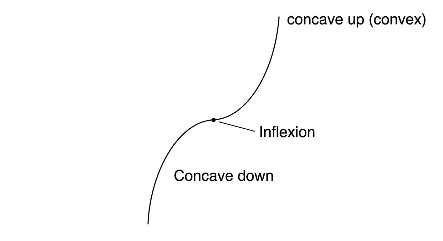
Concave up (like a cup, $\cup$ ): the slope is increasing as you move to the right.
Concave down (like an upside-down cup, $\cap$ ): the slope is decreasing as you move to the right.

The point where the bending changes direction is called an inflection point.

A curve that is concave down on the left, concave up on the right, with the inflection point where the bending changes

The second derivative test for concavity

Let $f$ be twice differentiable on an interval $I$ .

Sign of $f''(x)$ on $I$	Shape of the graph
$f''(x)>0$	concave up
$f''(x)<0$	concave down

Why. $f''$ is the rate of change of the slope $f'$ . If $f''>0$ , the slope is increasing, so the curve bends upward.

Watch out. If $f''(x)=0$ (or is not defined), the point is only a possible inflection point. It is a real inflection point only if $f''$ changes sign there. For $f(x)=x^4$ , $f''(0)=0$ but $f''$ is positive on both sides, so $0$ is not an inflection point.

Method

Find $f''(x)$ .
Solve $f''(x)=0$ (and note where $f''$ is not defined) to get the points where the sign may change.
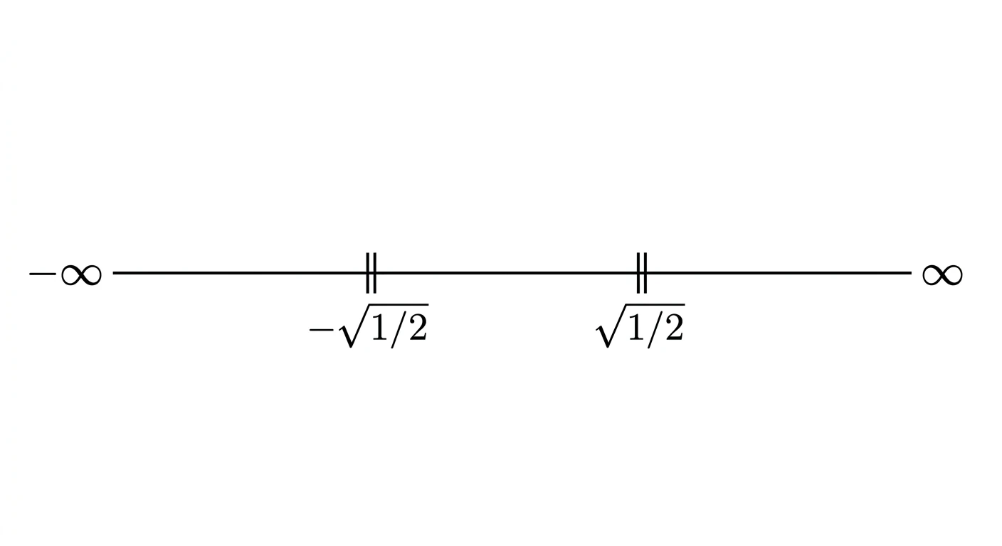
Check the sign of $f''$ in each interval between these points (a sign chart on a number line helps here).
Write the concavity, and mark the inflection points where the sign changes.

Examples

1. $f(x)=x^3-3x^2+4$

f'(x)=3x^2-6x,\qquad f''(x)=6x-6=6(x-1)

$f''<0$ for $x<1$ and $f''>0$ for $x>1$ .

Concave down on $(-\infty,\,1)$ .
Concave up on $(1,\,\infty)$ .
Inflection point at $x=1$ .

2. $f(x)=x^3-6x^2+9x+1$

f'(x)=3x^2-12x+9,\qquad f''(x)=6x-12=6(x-2)

Concave down on $(-\infty,\,2)$ .
Concave up on $(2,\,\infty)$ .
Inflection point at $x=2$ .

3. $f(x)=\ln x$ , for $x>0$

f'(x)=\frac1x,\qquad f''(x)=-\frac1{x^2}<0\ \text{ for all }x>0

Concave down on $(0,\,\infty)$ , with no inflection points.

4. $f(x)=e^{-x^2}$

\begin{aligned} f'(x)&=-2x\,e^{-x^2}\\ f''(x)&=-2e^{-x^2}+(-2x)(-2x)\,e^{-x^2}=2e^{-x^2}\,(2x^2-1) \end{aligned}

Since $e^{-x^2}>0$ always, the sign of $f''$ is the sign of $2x^2-1$ . It is $0$ when $x^2=\tfrac12$ , i.e. $x=\pm\tfrac1{\sqrt2}$ .

Number line with the points minus root half and root half marked, splitting the line into three intervals

Interval	$2x^2-1$	$f''$	Shape
$\left(-\infty,\,-\tfrac1{\sqrt2}\right)$	$+$	$+$	concave up
$\left(-\tfrac1{\sqrt2},\,\tfrac1{\sqrt2}\right)$	$-$	$-$	concave down
$\left(\tfrac1{\sqrt2},\,\infty\right)$	$+$	$+$	concave up

Inflection points at $x=\pm\dfrac1{\sqrt2}$ . (This is the bell curve: it bends down near the top and bends up on the two sides.)

5. $f(x)=e^x-x^2$

f'(x)=e^x-2x,\qquad f''(x)=e^x-2

Solve $f''=0$ : $\;e^x=2\Rightarrow x=\ln2$ (since $e^{\ln2}=2$ ).

For $x<\ln2$ : $e^x<2$ , so $f''<0$ → concave down on $(-\infty,\,\ln2)$ .
For $x>\ln2$ : $e^x>2$ , so $f''>0$ → concave up on $(\ln2,\,\infty)$ .
Inflection point at $x=\ln2$ .

Page 19 of 19

Practice questions and formula sheet

Practice questions

Try these without looking at the answers. The answers are given below.

A. Limits

$\displaystyle\lim_{x\to2}\frac{x^2-4}{x-2}$
$\displaystyle\lim_{x\to0}\frac{\sqrt{x+9}-3}{x}$
$\displaystyle\lim_{x\to\infty}\frac{5x^3-x}{2x^3+7}$
$\displaystyle\lim_{x\to0}x\cos\frac1x$

B. Differentiation. Use implicit differentiation to find $\dfrac{dy}{dx}$ :

$x^3y+xy^3=6$
$y^2=\dfrac{x-1}{x+1}$

C. First and second derivatives

$r=\dfrac1{3s^2}-\dfrac5{2s}$
$y=4-2x-x^{-3}$
$y=\left(\dfrac{1+3z}{3z}\right)(3-z)$
$y=\dfrac{(\theta-1)(\theta^2+\theta+1)}{\theta^3}$

D. First derivatives

$y=(5-2x^2)(2x^3-3x+4)$
$y=(1+x^2)\left(x^{3/4}-x^{-3}\right)$
$y=\dfrac{\sqrt{4s}-9}{\sqrt{4s}+9}$

Answers

$4$ . Factorise: $\frac{(x-2)(x+2)}{x-2}=x+2\to4$ .
$\tfrac16$ . Conjugate: $\frac{x}{x(\sqrt{x+9}+3)}=\frac1{\sqrt{x+9}+3}\to\frac16$ .
$\tfrac52$ . Same degree: ratio of leading coefficients.
$0$ . Sandwich: $-|x|\le x\cos\frac1x\le|x|$ .
$\dfrac{dy}{dx}=-\dfrac{3x^2y+y^3}{x^3+3xy^2}$
$\dfrac{dy}{dx}=\dfrac{1}{y\,(x+1)^2}$
$r'=-\dfrac{2}{3s^3}+\dfrac{5}{2s^2}$ , $\quad r''=\dfrac{2}{s^4}-\dfrac{5}{s^3}$
$y'=-2+3x^{-4}$ , $\quad y''=-12x^{-5}$
Expand first: $y=\dfrac1z+\dfrac83-z$ . So $y'=-\dfrac1{z^2}-1$ , $\quad y''=\dfrac2{z^3}$
Expand first: $y=1-\theta^{-3}$ . So $y'=3\theta^{-4}$ , $\quad y''=-12\theta^{-5}$
$y'=-20x^4+48x^2-16x-15$
$y'=\tfrac{11}{4}x^{7/4}+\tfrac34x^{-1/4}+x^{-2}+3x^{-4}$
$y'=\dfrac{18}{\sqrt s\,\left(2\sqrt s+9\right)^2}$

Study tip. In 9 and 10, if you expand or simplify before differentiating, you can use the easy power rule instead of the product or quotient rule.

Formula sheet

Limits


Definition	$\lim_{x\to c}f(x)=L$ means $f(x)\to L$ as $x\to c$ ( $x\neq c$ )
Exists only if	left limit $=$ right limit
Polynomials	$\lim_{x\to c}P(x)=P(c)$
Rational	$\lim_{x\to c}\dfrac{P}{Q}=\dfrac{P(c)}{Q(c)}$ if $Q(c)\ne0$
$0/0$	factorise and cancel, or multiply by the conjugate
Sandwich	$g\le f\le h$ and $g,h\to L$ $\Rightarrow$ $f\to L$
At infinity	divide by the highest power; $\dfrac1{x^n}\to0$
Standard limits	$\dfrac{\sin h}{h}\to1$ , $\ \dfrac{\ln(1+h)}{h}\to1$ as $h\to0$

Continuity

$f$ is continuous at $a$ when $f(a)$ exists, $\lim_{x\to a}f(x)$ exists, and they are equal. Left- and right-continuity use $\lim_{x\to a^-}$ and $\lim_{x\to a^+}$ .

Derivatives

f'(a)=\lim_{h\to0}\frac{f(a+h)-f(a)}{h}

Rule	Formula
Power	$(x^n)'=nx^{n-1}$
Product	$(fg)'=fg'+gf'$
Quotient	$\left(\dfrac fg\right)'=\dfrac{gf'-fg'}{g^2}$
Chain	$\dfrac{dy}{dx}=\dfrac{dy}{du}\cdot\dfrac{du}{dx}$
Implicit	differentiate both sides; every $y$ -term gets a factor $\dfrac{dy}{dx}$

$f$	$\sqrt x$	$\dfrac1x$	$e^x$	$\ln x$	$\sin x$	$\cos x$	$\tan x$
$f'$	$\dfrac1{2\sqrt x}$	$-\dfrac1{x^2}$	$e^x$	$\dfrac1x$	$\cos x$	$-\sin x$	$\sec^2x$

Applications


Tangent at $(x_0,y_0)$	$y-y_0=f'(x_0)(x-x_0)$
Normal at $(x_0,y_0)$	$y-y_0=-\dfrac{1}{f'(x_0)}(x-x_0)$
Linearization at $a$	$L(x)=f(a)+f'(a)(x-a)$
Concave up	$f''>0$
Concave down	$f''<0$
Inflection point	$f''$ changes sign

Module 1 at a glance

What you will be able to do

How to use these notes

Where each topic sits

Limits of function values

The idea

Example: a hole in the graph

Two simple limits to remember

When a limit does not exist

Limit laws

Polynomials and rational functions: just put the value

Example 1. Substitution works

Example 2. Root of an expression

Example 3. Substitution fails (the 0/00/00/0 case)

Finding limits: a method with the same first step every time

Step 0: try substitution

Technique A: factorise and cancel

Technique B: multiply by the conjugate

Technique C: simplify a fraction inside a fraction

Solved limit problems

Group 1: direct substitution

Group 2: 0/00/00/0, so factorise

Group 3: the denominator tends to 000 but the numerator does not

Group 4: roots, so use the conjugate

Group 5: fraction inside a fraction

The sandwich (squeeze) theorem

The idea

Example 1: bounds are given

Example 2: find the bounds yourself

Example 3: a root between two roots

Example 4: one-sided bound

Limits at infinity

The idea

Method for rational functions

Example 1

Example 2

Example 3 (take out the highest power as a common factor)

Shortcut: compare the degrees

Continuity

The idea

Definition

Example 1: f(x)=x2f(x)=x^2f(x)=x2 at x=3x=3x=3

Example 2: f(x)=1xf(x)=\dfrac1xf(x)=x1​ at x=1x=1x=1 and at x=0x=0x=0

A continuous function

Where is a function continuous?

Practice

One-sided limits and one-sided continuity

Notation

One-sided continuity

How to check in 3 steps

Example 1. Left-continuity at x=2x=2x=2

Example 2. Right-continuity at x=−1x=-1x=−1

Example 3. Right-continuity at x=3x=3x=3

Example 4. Left-continuity at x=1x=1x=1

The derivative

The idea

Method for first-principle questions

Examples

1. f(x)=x2f(x)=x^2f(x)=x2 at x=2x=2x=2

2. f(x)=xf(x)=\sqrt xf(x)=x​ at x=4x=4x=4

3. f(x)=3x2+2xf(x)=3x^2+2xf(x)=3x2+2x at x=1x=1x=1

4. f(x)=1xf(x)=\dfrac1xf(x)=x1​ at x=2x=2x=2

5. f(x)=sin⁡xf(x)=\sin xf(x)=sinx at x=0x=0x=0

6. f(x)=ln⁡xf(x)=\ln xf(x)=lnx at x=1x=1x=1

Rules of differentiation

Basic rules

Standard derivatives to remember

Worked examples

Higher-order derivatives

The idea

Examples

Instantaneous rate of change

The idea

Examples

The chain rule

The idea

Method

Examples

Chain rule combined with other rules

Implicit differentiation

Example 3. Substitution fails (the $0/0$ case)

Group 2: $0/0$ , so factorise

Group 3: the denominator tends to $0$ but the numerator does not

Example 1: $f(x)=x^2$ at $x=3$

Example 2: $f(x)=\dfrac1x$ at $x=1$ and at $x=0$

Example 1. Left-continuity at $x=2$

Example 2. Right-continuity at $x=-1$

Example 3. Right-continuity at $x=3$

Example 4. Left-continuity at $x=1$

1. $f(x)=x^2$ at $x=2$

2. $f(x)=\sqrt x$ at $x=4$

3. $f(x)=3x^2+2x$ at $x=1$

4. $f(x)=\dfrac1x$ at $x=2$

5. $f(x)=\sin x$ at $x=0$

6. $f(x)=\ln x$ at $x=1$