Mathematics for Information Science 1. Module 4, lagrange multipliers to linear programming.

Page 1 of 14

Module 4 at a glance

In Modules 2 and 3 we used derivatives to study functions. In Module 4 we use them, along with a little geometry, to find the best choice: the largest profit, the smallest cost, the shortest distance.

1. Lagrange multipliers. Find the maximum or minimum of $f(x,y)$ when $x$ and $y$ are connected by a condition such as $x^2+y^2=1$. There can be one condition (constraint) or two.
2. Linear programming. Optimise a linear objective like $z=3x_1+5x_2$ when the variables must satisfy some linear inequalities. Write word problems in mathematical form, and then solve them by the graphical method.
3. Gradient descent (steepest descent). A step-by-step numerical method that moves downhill to a minimum, using the gradient from Module 3.

What you will be able to do

• Set up the Lagrange function $L=f+\lambda g$ and solve the system $\nabla L=0$.
• Find the point on a plane that is closest to the origin, the largest area for a fixed perimeter, and similar problems.
• Solve problems with two constraints using two multipliers $\lambda$ and $\mu$.
• Convert a word problem into a linear programming problem (LPP).
• Draw the feasible region of a two-variable LPP, find its corner points and choose the optimal one.
• Identify infeasible, unbounded and multiple-optimum problems.
• Do gradient descent iterations by hand.

How to use these notes

• Every topic has the same shape: idea → method → worked examples → common mistakes.
• Try each worked example yourself before reading the solution.
• Green boxes hold key ideas. Amber boxes marked Watch out show the mistakes that make you lose marks. Boxes marked Note on the source show where the handwritten class notes were corrected.
• The last page has practice questions with answers and a formula sheet.

Where each topic sits

Before you start. You should know partial derivatives and the gradient (Modules 2 and 3), how to solve simultaneous linear equations, and how to draw straight lines using their intercepts.

Page 2 of 14

Lagrange multipliers

The idea

In Module 3 we found extreme values of $f(x,y)$ where $x$ and $y$ could take any values. Many times they are not free: a fence of fixed length, a point that must stay on a circle, a budget that must be spent fully. Such a condition is called a constraint, and it is written as

We want the largest or smallest value of $f$ among the points that satisfy the constraint.

Key idea. At a constrained maximum or minimum, the level curve of $f$ just touches the constraint curve $g=0$. Curves that touch have parallel normals, so $\nabla f$ and $\nabla g$ are parallel: $\nabla f=-\lambda\nabla g$ for some number $\lambda$. This is the Lagrange multiplier.

Method

1. Write the function $f(x,y)$, and write the constraint in the form $g(x,y)=0$.
2. Build the Lagrange function

3. Put all its partial derivatives equal to zero:

That is,

The third equation is just the constraint itself.

4. Solve for $x$, $y$ (and $\lambda$). The solutions are the critical points.
5. Find $f$ at every critical point. On a closed, bounded constraint curve (a circle, an ellipse) the largest value is the maximum and the smallest value is the minimum.

Solving tip. The usual trick: find $\lambda$ from the first two equations, put the two expressions equal (this removes $\lambda$), and put the resulting relation between $x$ and $y$ in the constraint.

First example

Example 1. Find the extreme value of $f(x,y)=x^2+y^2$ subject to $x+y=1$.

Here $g(x,y)=x+y-1=0$ and

From (1) and (2), $\lambda=-2x=-2y$, so $x=y$. Putting this in (3): $2x=1$, so

This is the minimum. $x^2+y^2$ is the square of the distance from the origin, and $\left(\tfrac12,\tfrac12\right)$ is the point on the line $x+y=1$ that is nearest to the origin.

Note on the source. The class notes asked to "maximise" $x^2+y^2$ on $x+y=1$. There is no maximum, because points on the line far from the origin make $x^2+y^2$ as large as we like. The only critical point $\left(\tfrac12,\tfrac12\right)$ gives the minimum value $\tfrac12$.

Watch out. The Lagrange method gives only possible points. Decide whether each point is a maximum or a minimum by comparing the values. Remember that on an unbounded constraint (a line, a plane), one of the two may not exist.

Page 3 of 14

Lagrange multipliers: worked examples

Example 1. Find the maximum and minimum of $f(x,y)=xy$ subject to $x^2+y^2=1$.

From (1), $\lambda=-\dfrac{y}{2x}$; from (2), $\lambda=-\dfrac{x}{2y}$. Equating them, $y^2=x^2$. Then (3) gives $2x^2=1$, so $x=\pm\dfrac1{\sqrt2}$, $y=\pm\dfrac1{\sqrt2}$: four critical points.

Maximum $\tfrac12$ at the first pair, minimum $-\tfrac12$ at the second pair.

Example 2. Maximise $f(x,y)=xy$ subject to $x^2+4y^2=4$.

From (1), $\lambda=-\dfrac{y}{2x}$; from (2), $\lambda=-\dfrac{x}{8y}$. Equating and cross-multiplying:

Put $x^2=4y^2$ in (3): $4y^2+4y^2=4$, so $y^2=\tfrac12$ and $y=\pm\dfrac1{\sqrt2}$, $x=\pm\sqrt2$.

The maximum is $1$ at $\left(\sqrt2,\tfrac1{\sqrt2}\right)$ and $\left(-\sqrt2,-\tfrac1{\sqrt2}\right)$.

Note on the source. The class notes went from $8y^2=2x^2$ to "$y=x/4$", where the square root was taken wrongly (it should be $x=\pm2y$). Then they found $xy$ at $\left(\frac4{\sqrt5},\frac1{\sqrt5}\right)$ by adding the coordinates and got $\sqrt5$. That point does lie on the ellipse, but $xy$ there is only $\frac45$. The correct maximum is $1$.

Example 3. Find the extreme values of $f(x,y)=xy$ subject to $x^2+y^2=10$.

Exactly as in Example 1: $L_x=y+2\lambda x=0$ and $L_y=x+2\lambda y=0$ give $x^2=y^2$, and the constraint gives $2x^2=10$, so $x=\pm\sqrt5$, $y=\pm\sqrt5$.

Maximum $5$, minimum $-5$.

Note on the source. One line of the handwritten table wrote $f(-\sqrt5,\sqrt5)=5$. It should be $-5$. The final conclusion in the notes was correct.

Example 4. Find the maximum and minimum of $f(x,y)=3x+4y$ on the circle $x^2+y^2=1$.

Put this in the constraint:

• $\lambda=-\tfrac52$: $x=\tfrac35$, $y=\tfrac45$, and $f=\tfrac95+\tfrac{16}5=\mathbf{5}$ (maximum).
• $\lambda=\tfrac52$: $x=-\tfrac35$, $y=-\tfrac45$, and $f=-\tfrac95-\tfrac{16}5=\mathbf{-5}$ (minimum).

Note on the source. In the copied notes, the page was blank after the value $-5$. The maximum $5$ at $\left(\tfrac35,\tfrac45\right)$ is completed here.

Watch out. When you divide by $x$ or $y$ to get $\lambda$, you are assuming that they are not zero. Check separately whether $x=0$ or $y=0$ can satisfy the equations. (In these examples it cannot, because then the other variable would also be $0$, and that point is not on the curve.)

Page 4 of 14

Lagrange multipliers: applications

The method works in the same way with three variables: $L=f(x,y,z)+\lambda g(x,y,z)$ and four equations $L_x=L_y=L_z=L_\lambda=0$.

Example 1. Closest point on a plane. Find the point $P(x,y,z)$ on the plane $2x+y-z-5=0$ that is closest to the origin.

The distance is $d=\sqrt{x^2+y^2+z^2}$. Minimising $d$ is the same as minimising $d^2$, which has no square root, so take

Put these in the plane equation:

so

Check. The distance from the origin to $ax+by+cz=k$ is $\dfrac{|k|}{\sqrt{a^2+b^2+c^2}}=\dfrac{5}{\sqrt6}$. $\checkmark$

Note on the source. The notes wrote "$x=-\lambda/2$" from $2x+2\lambda=0$, but it should be $x=-\lambda$. The next lines actually used $x=-\lambda$, so the final point $\left(\tfrac53,\tfrac56,-\tfrac56\right)$ is correct.

Example 2. Find the minimum of $f(x,y,z)=x^2+y^2+z^2$ subject to $x+y+z=9$.

$L_x=2x+\lambda=0$, $L_y=2y+\lambda=0$, $L_z=2z+\lambda=0$ give $x=y=z=-\dfrac\lambda2$. The constraint gives $3x=9$, so $x=y=z=3$ and $\lambda=-6$:

Note on the source. The question of this example was missing in the copied notes. Only the working "$\lambda=-6$, $x=y=z=3$, $f=27$" was available. The constraint $x+y+z=9$ gives exactly that working.

Example 3. Largest rectangle. A rectangle has perimeter $20\ \text{m}$. Find the dimensions that maximise its area.

Let the length be $x$ and the breadth be $y$. Maximise $f=xy$ subject to $2(x+y)=20$, that is $g=x+y-10=0$.

The constraint gives $-2\lambda=10$, so $\lambda=-5$ and

The best rectangle is a square.

Note on the source. One line of the notes read "$x-x-10=0$". It should be $x+x-10=0$ (the next line, $-\lambda-\lambda-10=0$, is correct).

Watch out. When the quantity to optimise is a distance, minimise $d^2$ instead of $d$. The square root only makes the derivatives difficult and does not change the place where the minimum comes.

Page 5 of 14

Lagrange multipliers with two constraints

Method

To optimise $f(x,y,z)$ subject to two constraints $g(x,y,z)=0$ and $h(x,y,z)=0$, use one multiplier for each:

and solve the five equations

The last two are the constraints themselves.

Key idea. Each constraint takes away one degree of freedom. In three variables with two constraints, the allowed points form a curve (usually a line, where two planes meet), and we optimise $f$ along it.

Examples

Example 1. Find the extreme value of $f(x,y)=x^2+y^2$ subject to $x+y=1$ and $x-y=1$.

Adding (3) and (4): $2x=2$, so $x=1$, and then $y=0$. From (1) and (2): $2+\lambda+\mu=0$ and $\lambda-\mu=0$, so $\lambda=\mu=-1$.

Two lines in the plane meet at a single point, so $(1,0)$ is the only point that satisfies both constraints, and $1$ is the only value $f$ can take.

Example 2. Find the extreme value of $f(x,y,z)=x^2+y^2+z^2$ subject to $x+y+z=3$ and $x-y+z=1$.

• (4) $-$ (5): $2y-2=0$, so $y=1$.
• (1) and (3) give $2x=-(\lambda+\mu)=2z$, so $x=z$.
• (4) then gives $2x+1=3$, so $x=z=1$.

The critical point is $(1,1,1)$ with

This is the minimum: the two planes meet in a line, and $(1,1,1)$ is the point on that line nearest to the origin. There is no maximum, because the line goes to infinity.

Example 3. Find the extremum of $f(x,y,z)=x^2+y^2+z^2$ subject to $x+y+z=1$ and $x-y=0$.

• (5): $x=y$.
• (1) $-$ (2): $2(x-y)+2\mu=0$, so $\mu=0$.
• Then (1) and (3) give $2x=-\lambda=2z$, so $x=z$.
• (4): $3x=1$, so $x=y=z=\tfrac13$.

Note on the source. The copied page with Examples 2 and 3 was not clear. The working above is rebuilt from the equations that were readable, and both answers have been checked again: $(1,1,1)$ with value $3$, and $\left(\tfrac13,\tfrac13,\tfrac13\right)$ with value $\tfrac13$.

Watch out. Number your equations and write which ones you are combining. With five equations it is easy to miss one, and a missing equation usually gives a wrong point.

Page 6 of 14

Linear programming: the terms

The idea

A linear programming problem (LPP) asks for the best value of a linear function when the variables must obey several linear inequalities. It models production planning, diets, staffing, transport and many other decisions.

The parts of an LPP

Constraints come in three types:

General form

subject to

Kinds of solution

• Feasible solution: any values of the variables that satisfy all the constraints, including non-negativity. The set of all feasible solutions is the feasible region.
• Basic feasible solution: with $n$ variables and $m$ equality constraints, put $n-m$ of the variables equal to $0$ and solve for the rest. If the result is feasible, it is a basic feasible solution. In the graph, these are the corner points of the feasible region.
• Optimal solution: a feasible solution that gives the largest value (for maximise) or the smallest value (for minimise) of the objective.

Each inequality is a half-plane

A single linear inequality in two variables is satisfied on one side of its boundary line. To find which side, test a point not on the line, usually the origin: if $(0,0)$ satisfies the inequality, shade the side containing the origin; otherwise shade the other side. The feasible region is where all the shaded sides overlap.

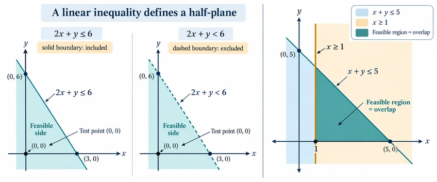
Watch out. "$\le$" does not always mean "shade below". For $x_1-3x_2\ge-6$, the origin gives $0\ge-6$, which is true, so the side of the origin is shaded even though the line slopes upward. Always test a point.

Page 7 of 14

Formulating an LPP from a word problem

Method

1. Name the decision variables: which quantities can we choose? Write what each one means.
2. Write the objective function: the profit, cost or number to be maximised or minimised, in terms of the variables.
3. Write one constraint for each limited resource or requirement. "Available" or "at most" gives $\le$. "At least" or "required" gives $\ge$.
4. Add non-negativity: $x_1,x_2,\dots\ge0$.

Examples

Example 1. Manufacturing. A factory makes products $P_1$ and $P_2$, with profit Rs 3 and Rs 5 per unit. $P_1$ needs 1 unit of resource 1 and 2 units of resource 2; $P_2$ needs 2 units of resource 1 and 1 unit of resource 2. Only 4 units of resource 1 and 6 units of resource 2 are available. Write the LPP to maximise the profit.

Let $x_1$, $x_2$ be the numbers of units of $P_1$ and $P_2$ produced.

subject to

(It is solved on the practice page: the best profit is $\tfrac{34}{3}$ at $x_1=\tfrac83$, $x_2=\tfrac23$.)

Example 2. Diet problem. A hospital diet must provide at least 2000 calories, 50 g of protein and 300 g of carbohydrate per day, at minimum cost. Food 1 costs Rs 3 per unit and gives 500 cal, 20 g protein and 30 g carbohydrate. Food 2 costs Rs 4 per unit and gives 600 cal, 30 g protein and 40 g carbohydrate. Write the LPP.

Let $x_1$, $x_2$ be the units of food 1 and food 2 per day.

subject to

(It is solved graphically on the "word problems" page.)

Example 3. Staff scheduling. A company needs at least 5 employees from 8 am to 12 noon, 3 from 12 noon to 4 pm, and 4 from 4 pm to 8 pm. Each employee works an 8-hour shift starting at 8 am, 12 noon or 4 pm. Minimise the number of employees.

Let $x_1$, $x_2$, $x_3$ be the numbers starting at 8 am, 12 noon and 4 pm. A person starting at 8 am works from 8 am to 4 pm, so covers the first two periods. A person starting at noon covers the second and third periods. A person starting at 4 pm covers the third period.

subject to

The minimum is $9$ employees, for example $x_1=5$, $x_2=0$, $x_3=4$: the first constraint forces $x_1\ge5$ and the third forces $x_2+x_3\ge4$.

Note on the source. The handwritten question said employees "can't start" at 8 am, 12 noon or 4 pm, and named $x_1,x_2,x_3$ by the four-hour periods. The constraints in the notes make sense only if shifts start at those times, so we have used that meaning here.

Watch out. Write what each variable means, with units. Most mistakes in writing the LPP come from a variable whose meaning changes in the middle of the working.

Page 8 of 14

The graphical method

The idea

With two decision variables, we can draw the feasible region. For a linear objective, the lines $z=\text{constant}$ are parallel. If we move them in the direction in which $z$ increases, the last point of the region that they touch is a corner.

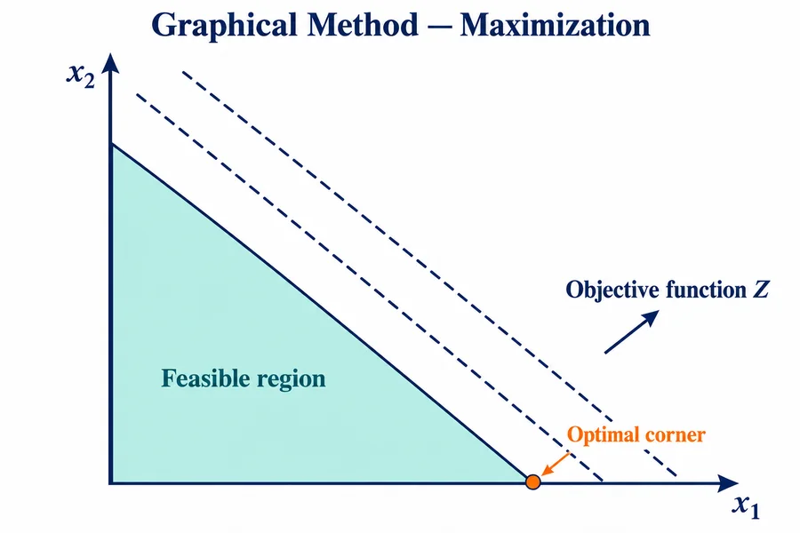
Key idea (corner-point theorem). If an LPP has an optimal solution, then one occurs at a corner point (vertex) of the feasible region. So we only need to find $z$ at the corners.

Method

1. Change each inequality to an equation and draw the line, using its two intercepts (put $x_1=0$, and then $x_2=0$).
2. Shade the side of each line that satisfies the inequality (test the origin). Also include $x_1,x_2\ge0$.
3. The common part is the feasible region. Write its corner points. Find each one by solving the equations of the two lines that meet there.
4. Find $z$ at every corner. The largest (or smallest) value is the optimum.

Examples

Example 1. Maximise $z=3x_1+4x_2$ subject to $4x_1+2x_2\le80$, $2x_1+5x_2\le180$, $x_1,x_2\ge0$.

Intercepts: $4x_1+2x_2=80$ passes through $(20,0)$ and $(0,40)$; $2x_1+5x_2=180$ passes through $(90,0)$ and $(0,36)$.

The two lines meet where $4x_1+2x_2=80$ and $2x_1+5x_2=180$. Multiply the second by 2 to get $4x_1+10x_2=360$. Subtracting the first, $8x_2=280$, so $x_2=35$ and $x_1=\tfrac52$.

Maximum $z=147.5$ at $x_1=2.5$, $x_2=35$.

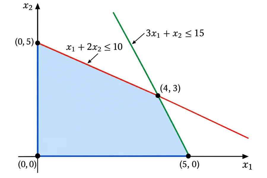
Example 2. Maximise $z=3x+2y$ subject to $x+2y\le10$, $3x+y\le15$, $x,y\ge0$.

Intercepts: $x+2y=10$ through $(10,0)$ and $(0,5)$; $3x+y=15$ through $(5,0)$ and $(0,15)$. They meet where $6x+2y=30$ and $x+2y=10$. Subtracting, $5x=20$, so $x=4$, $y=3$.

Maximum $z=18$ at $(4,3)$.

Watch out. An intercept of a constraint line is a corner only if it satisfies every other constraint. In Example 2, $(10,0)$ is on $x+2y=10$ but does not satisfy $3x+y\le15$, so it is not a corner.

Page 9 of 14

Graphical method: more examples

Example 1. Maximise $z=15x_1+10x_2$ subject to $4x_1+6x_2\le360$, $3x_1\le180$, $5x_2\le500$, $x_1,x_2\ge0$.

The constraints say $4x_1+6x_2\le360$ (through $(90,0)$ and $(0,60)$), $x_1\le60$, and $x_2\le100$. The last one is never the deciding one, because $4x_1+6x_2\le360$ already forces $x_2\le60$.

The line $x_1=60$ meets $4x_1+6x_2=360$ at $240+6x_2=360$, so $x_2=20$.

Maximum $z=1100$ at $x_1=60$, $x_2=20$.

Note on the source. The class notes listed the corners as $(0,0)$, $(90,0)$, $(60,20)$, $(40,30)$, $(0,40)$ and chose $1350$ at $(90,0)$. But $(90,0)$ does not satisfy $3x_1\le180$, the point $(40,30)$ is not where any two constraint lines meet, and $(0,40)$ is not on any boundary. The correct corners are those in the table, and the maximum is $1100$.

Example 2. Maximise $z=2x+3y$ subject to $x+y\le30$, $3\le y\le12$, $x-y\ge0$, $0\le x\le20$.

The region lies between the horizontal lines $y=3$ and $y=12$, to the right of the line $y=x$ (because $x\ge y$), to the left of $x=20$, and below $x+y=30$. Its corners are:

• $y=3$ meets $y=x$ at $A(3,3)$ and meets $x=20$ at $B(20,3)$.
• $x=20$ meets $x+y=30$ at $C(20,10)$.
• $x+y=30$ meets $y=12$ at $D(18,12)$.
• $y=12$ meets $y=x$ at $E(12,12)$.

Maximum $z=72$ at $(18,12)$. (The minimum, if asked, is $15$ at $(3,3)$.)

Note on the source. The notes used $E(3,12)$ as a corner, with $z=42$. That point does not satisfy $x\ge y$. The correct corner is $E(12,12)$ with $z=60$. The maximum does not change.

Example 3. Maximise $f=5x_1+25x_2$ subject to $x_1-3x_2\ge-6$, $x_1+x_2\le6$, $x_1,x_2\ge0$.

The line $x_1-3x_2=-6$ passes through $(0,2)$ and $(-6,0)$, and the origin satisfies $0\ge-6$, so the feasible side is below this line that goes up. The line $x_1+x_2=6$ passes through $(6,0)$ and $(0,6)$. The two lines meet where $x_1=3x_2-6$ and $x_1+x_2=6$: $4x_2=12$, so $x_2=3$, $x_1=3$.

Maximum $f=90$ at $(3,3)$.

Note on the source. The notes gave the $x_2$-intercept of $x_1-3x_2=-6$ as $(0,-2)$. It is $(0,2)$ (put $x_1=0$: $-3x_2=-6$). The corner $D(0,2)$ in the notes was correct.

Page 10 of 14

Word problems solved graphically

Example 1. Chairs and tables. A manufacturer makes chairs and tables on machines $A$ and $B$. A chair needs 2 hours on $A$ and 6 hours on $B$; a table needs 5 hours on $A$ and 1 hour on $B$. Machine $A$ is available 16 hours a day and machine $B$ 30 hours. The profit is Rs 2 per chair and Rs 10 per table. Write the LPP and solve it.

Let $x_1$ chairs and $x_2$ tables be made per day.

subject to

Intercepts: $2x_1+5x_2=16$ through $(8,0)$ and $\left(0,\tfrac{16}5\right)$; $6x_1+x_2=30$ through $(5,0)$ and $(0,30)$.

The two lines meet here: from the second, $x_2=30-6x_1$; then $2x_1+150-30x_1=16$, so $x_1=\tfrac{134}{28}=\tfrac{67}{14}\approx4.79$ and $x_2=\tfrac97\approx1.29$.