
Page 1 of 25
Module 1 at a glance
This module answers two questions about electrons in solids.
- Why does a copper wire conduct, glass does not, and silicon conducts only a little? We build the answer in three steps. First, a classical picture, in which the electrons in a metal behave like a gas. Then, a quantum correction, in which electrons follow the Pauli exclusion principle and Fermi–Dirac statistics. Finally, band theory, in which the regular arrangement of atoms in a crystal splits the electron energy levels into bands, with gaps between the bands.
- Why do some materials lose all their resistance when cooled? This is superconductivity. We study its critical temperature, its critical magnetic field, the Meissner effect, the two types of superconductor, the BCS theory that explains it, and its applications.
KTU syllabus. Electrical conductivity: classical free electron theory, electrical conductivity in metals, Fermi–Dirac distribution, variation of the Fermi function with temperature, Fermi energy, energy bands, classification of materials into conductor, semiconductor and insulator. Superconductivity: superconductivity, transition temperature, critical field, Meissner effect, Type I and Type II superconductors, BCS theory, applications of superconductors.
What you will be able to do
- Define and use electric field, current density, drift velocity, relaxation time, mean free path, mobility, conductivity and resistivity, with their units.
- Derive from the classical free electron theory in two ways, and write the factors that affect conductivity.
- Write the assumptions, successes and failures of the classical theory, and explain how the quantum free electron theory improves it.
- Write the Fermi–Dirac function, find its value at and at higher temperatures, draw its graph, and define the Fermi energy.
- Explain how energy bands form, and use band diagrams to classify conductors, semiconductors and insulators.
- Describe the properties of superconductors: zero resistance, persistent currents, critical temperature, critical field, flux quantisation and the isotope effect.
- Derive from the Meissner effect, and distinguish Type I from Type II superconductors.
- Explain Cooper pairs and the BCS theory, and list the applications of superconductors.
- Solve the standard numerical problems on conductivity, the Fermi function, the Fermi energy and the critical field.
How to use these notes
- Each topic is a short page: idea → explanation or derivation → worked example → common mistakes.
- Green boxes show key ideas and definitions. Amber boxes marked Watch out show mistakes that make you lose marks. Boxes marked Note on the source show where the lecture notes were corrected.
- Try each numerical problem yourself before reading the solution. Every answer has been checked again.
- The last page has practice problems with answers, a list of exam-type questions and a formula sheet.
Where each topic sits
| Part | Pages |
|---|---|
| Basic ideas | Key terms, Ohm's law and conductivity |
| Classical theory | Assumptions and electron motion, drift velocity and the conductivity formula, factors affecting conductivity, failures |
| Quantum theory | Quantum free electron theory, Fermi–Dirac statistics, variation with temperature, Fermi energy |
| Band theory | Formation of bands, band diagram, conductors, semiconductors and insulators |
| Numerical problems | Conductivity, Fermi function and Fermi energy |
| Superconductivity | Discovery and transition temperature, properties, review of magnetism, critical field, Meissner effect, Type I and II, BCS theory, applications |
Before you start. You should know Ohm's law, Newton's second law and the equation of motion , magnetic field and magnetic flux, and the exponential function with its inverse . You should also be comfortable with powers of ten, because almost every number in this module is either very large (electron density near ) or very small (times near ).
Page 2 of 25
Terms you need before you start
Every derivation in this module uses the same small set of quantities. First learn their meanings and units.
1. Electric field
The electric field is a vector field that tells the force a charge would feel at each point in space. It is defined as the force per unit charge:
where is the force experienced by a charge . Its unit is newton per coulomb, which is the same as volt per metre (V/m).
When a conductor is connected to a battery, the electric field pushes the free electrons and makes them flow. This gives an electric current. For a uniform wire of length with a voltage across it, the field inside is .
2. Current density
The current density is the electric current flowing per unit area of the cross-section of the conductor:
where is the current and is the cross-sectional area. Its unit is ampere per square metre ().
Current density is more useful than current in theory, because it does not depend on the size of the wire. A thick wire and a thin wire of the same metal in the same field have the same , even though the thick wire carries more current.
3. Drift velocity
Even without any applied field, the free electrons in a metal move at high speed in random directions because of their thermal energy. When a field is applied, the electrons get a slow average velocity in the direction opposite to the field, in addition to this random motion. This average velocity is the drift velocity .
Drift velocity is proportional to the electric field, and it is what produces the current. It is very small: typically to , compared with random speeds of about .
4. Relaxation time
The relaxation time is the average time between two successive collisions of an electron in the conductor. After each collision the electron loses the extra velocity it got from the field, and it starts accelerating again from the beginning.
Relaxation time decides how freely the electrons can move. A longer relaxation time means the electrons are accelerated for a longer time between collisions, so they drift faster and the conductivity is higher. Typical values in metals are about .
5. Mean free path
The mean free path is the average distance an electron travels between two successive collisions. It is related to the relaxation time through the average speed of the electrons:
The mean free path tells us how far an electron goes before it is scattered, so it also affects the conductivity of the material.
6. Mobility
The mobility of a charge carrier tells how easily it responds to an electric field. It is defined as the drift velocity per unit electric field:
Its unit is . In the classical theory (derived on a later page) , so mobility depends on the relaxation time. Higher mobility means the electrons move more freely when a field is applied.
7. Conductivity
Electrical conductivity tells how easily a material conducts electric current. It depends on the number of free electrons, their charge and their mobility:
The higher the conductivity, the more easily the material allows current to flow. Its unit is siemens per metre (S/m), also written mho/m or .
8. Resistivity
Resistivity is the reciprocal of conductivity. It tells how strongly a material opposes the flow of current:
Its unit is ohm metre (). Resistivity depends on the material and on its temperature. Materials with low resistivity (metals) are good conductors, and materials with high resistivity (insulators) resist the flow of current.
Summary table
| Quantity | Definition | Unit |
|---|---|---|
| Electric field | V/m | |
| Current density | A/m² | |
| Drift velocity | average velocity due to the field | m/s |
| Relaxation time | average time between collisions | s |
| Mean free path | average distance between collisions, | m |
| Mobility | m²/(V s) | |
| Conductivity | S/m | |
| Resistivity | m |
Watch out. Do not mix up current (a total, in amperes) with current density (per unit area, in A/m²). Also, do not confuse resistivity (a property of the material) with resistance (a property of a particular piece of it, which depends on its length and area).
Page 3 of 25
Ohm's law, resistivity and conductivity
Ohm's law
Electrical conductivity is a measure of how easily an electric current can pass through a material. When a current flows through a conductor, the voltage drop across it is given by Ohm's law:
where is the current in amperes, is the resistance in ohms and is the voltage drop in volts.
Resistance and resistivity
Consider an ideal conductor with uniform cross-section and uniform composition, so that the electric field and current density are constant and parallel everywhere inside it.
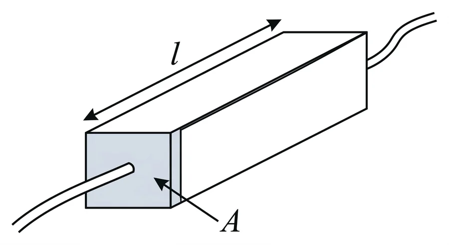
Experiments show that the resistance is directly proportional to the length and inversely proportional to the area :
The constant of proportionality is the electrical resistivity of the material, with SI unit . The conductivity is its reciprocal:
Point form of Ohm's law
If the shape is more complicated, or the resistivity changes from point to point, the current density and the field become functions of position. Then we use a more general, local statement. With the field at a point and the current density there, the conductivity at that point is
This is the point form of Ohm's law. It is true at each point of a material, whatever its shape.
The point form from
For a uniform conductor the point form follows directly from Ohm's law. Start from
Put in the first equation:
The field in a uniform conductor is , so can be replaced by :
Dividing by gives the current density:
So for a uniform conductor of area and length , the general expression becomes the familiar , and the two descriptions agree.
Classification of materials by conductivity
| Class | Typical conductivity | Examples |
|---|---|---|
| Conductors | about | metals and alloys |
| Semiconductors | to | silicon, germanium |
| Insulators | about and below | metal oxides, glasses, plastics |
The conductivities of real materials differ by more than twenty powers of ten. This is one of the widest ranges of any physical property. The theories on the next pages try to explain why.
Example
Example 1. A copper wire is long and has cross-section . Copper has resistivity . Find its resistance, and the field and current density when it carries .
Check with the point form: , and .
Watch out. Convert areas to square metres before putting the values: , not .
Page 4 of 25
Classical free electron theory (Drude–Lorentz)
The idea
The classical free electron theory was one of the earliest models to explain the electrical and thermal properties of metals. It was developed by Paul Drude in 1900 and later improved by Hendrik Lorentz, so it is also called the Drude–Lorentz theory.
Its main idea is that the valence electrons in a metal behave like the molecules of an ideal gas trapped in a box. The box is made by the fixed positive ions of the metal. The theory gave the base for understanding conduction in metals, but it also had important limitations that only quantum mechanics could remove.
Assumptions
- A metal is made of fixed ions and free electrons. The metal has positive ion cores, fixed in a regular lattice, and valence electrons that are free to move through the whole metal. The free electrons are not bound to any particular atom.
- Electrons are independent particles, like a gas. The free electrons are treated as independent particles moving inside the metal, just as gas molecules move inside a container. The positive ions are treated as fixed.
- Electrons follow Newtonian mechanics. Their motion is described by classical ideas: velocity, momentum, force and Newton's laws.
- Random thermal motion. The free electrons move randomly in all directions with speeds of about , and their speeds follow the Maxwell–Boltzmann distribution, as in the kinetic theory of gases.
- Collisions. Electrons collide with the ions (and with each other). Between collisions they travel in straight lines. The average time between collisions is the relaxation time , and the average distance is the mean free path . These collisions give the material its resistance.
- Response to a field. The velocity of an electron is decided by two things: the random thermal motion due to temperature, and the extra velocity due to the applied electric field.
- Carriers of charge and heat. The free electrons carry both charge and heat, so they are responsible for electrical and thermal conduction in metals.
Motion in the absence of a field: thermal motion
Without an applied field, each free electron moves at high speed in a straight line until it collides with an ion. Then it changes direction and moves again. Its path is a random zigzag.
Because the directions are random, for every electron moving in a particular direction there is, on average, another electron moving in the opposite direction. So the thermal motion gives no net flow of charge, and no current flows through the metal.
Motion when a field is applied: drift
Now connect the ends of a piece of metal to the terminals of a battery. An electric field is set up inside the metal. Each free electron feels a force in the direction opposite to the field (because it is negatively charged).
The electrons still move randomly and still collide, but along with the random motion, a slow net movement in one direction starts. This movement of electrons in one direction due to an electric field is called drift. The current is carried by the drift.
Key idea. The electrons in a metal move very fast, but in random directions, so on average they do not go anywhere. A field adds a small, steady drift to this random motion. The current comes only from the drift.
Orders of magnitude
| Typical value | |
|---|---|
| Random (thermal) speed | about |
| Drift speed | to |
| Relaxation time | about |
| Free electron density in a metal | about to |
Watch out. The drift speed is very small, so electricity does not "arrive" because individual electrons rush along the wire. The electric field is set up along the whole wire almost at once, and every free electron starts drifting at practically the same time.
Page 5 of 25
Drift velocity and the expression for conductivity
Drift velocity
When a field is applied, each free electron (charge , mass ) feels a force
The minus sign shows that the force on an electron is opposite to the field. By Newton's second law, , so the acceleration is
Electrons do not keep accelerating forever, because they collide frequently. Assume that after each collision an electron starts again from rest on average (). By the equation of motion , its velocity at a time after the collision is
The average time between collisions is the relaxation time . Taking gives the average velocity that the electron gets from the field. This is the drift velocity:
In magnitude, . The minus sign only shows that electrons drift against the field.
Current density from the drift (method 1)
Let be the number of free electrons per unit volume, called the free electron density or electron concentration. Consider a piece of metal of length and cross-section .
- The total number of free electrons in it is .
- Their total charge is .
- These electrons drift through the length in a time , so the current is
The term is the drift velocity , so
and the current density is
(With signs: , and since is itself negative, comes out in the direction of the field, as conventional current should.)
Expression for conductivity
Put (in magnitude) in :
Compare this with the point form of Ohm's law . The two are the same if
This is the classical expression for the electrical conductivity of a metal. The resistivity is its reciprocal, .
Second derivation via Ohm's law (method 2)
We get the same result from the macroscopic route on the previous page. From , and we found
From the microscopic route we found . Both describe the same current density in the same field, so the coefficients of must be equal. This again gives .
Mobility
The equation shows that the drift velocity is proportional to the field, . Write it as
where the constant is the electron mobility: the drift velocity per unit field,
Putting this in the conductivity formula,
Note on the source. One lecture set wrote , carrying the negative sign of the electron into the mobility. Mobility is normally written as a positive quantity, , and the direction of drift is stated separately.
Example
Example 1. A copper wire of cross-section carries . Copper has . Find the drift velocity.
That is about . An electron would take nearly two hours to drift one metre.
Watch out. In the charge is squared. One factor of comes from the force that causes the drift, and the other comes from the charge carried by each drifting electron.
Page 6 of 25
Factors affecting conductivity, and what the classical theory achieved
Factors affecting electrical conductivity in metals
From , the conductivity depends on the number of free electrons and on the relaxation time (which is related to the mean free path).
Number of free electrons . Metals have a high density of free electrons, and conductivity increases with the number of electrons available to carry current. Silver and copper conduct very well partly because of their high free electron density.
Mean free path. The longer an electron travels between collisions, the more it is accelerated and the higher the conductivity. At high temperatures electrons are scattered more often, by collisions with ions, with each other, and with the thermal vibrations of the lattice. So the mean free path becomes shorter and the conductivity falls.
Relaxation time . The longer the average time between collisions, the greater the mobility and the higher the conductivity.
Temperature.
- At low temperatures the thermal vibrations of the lattice (called phonons) are weak, so electrons are scattered less. Conductivity increases as temperature decreases.
- At high temperatures the lattice vibrates more strongly, electron–phonon scattering becomes more frequent, and conductivity decreases.
So in a metal the resistivity increases with temperature. Metals have a positive temperature coefficient of resistance.
Impurities and defects. Foreign atoms in the lattice and crystal defects (vacancies, dislocations, grain boundaries) scatter the free electrons. This reduces the relaxation time and therefore the conductivity. This is why alloys usually conduct less than the pure metals they are made from.
| Factor | Effect on |
|---|---|
| More free electrons | increases |
| Longer relaxation time or mean free path | increases |
| Higher temperature (metals) | decreases |
| Impurities and defects | decreases |
Importance of the classical theory
Even with its limitations, the classical free electron theory played an important role in the development of solid-state physics.
- It gave the base for understanding the electrical and thermal properties of metals.
- The model is simple, yet it explains basic phenomena such as electrical conductivity and Ohm's law.
- It gives the correct form of the Wiedemann–Franz law: the ratio of thermal conductivity to electrical conductivity is proportional to the temperature, , where is the Lorenz number.
- Its failures showed the need for quantum mechanics to explain the behaviour of electrons in solids. This led to more advanced theories such as the band theory of solids.
Transition to quantum models
The Drude–Lorentz model was a step towards the modern quantum theory of metals. In 1928 Arnold Sommerfeld improved the classical theory by using quantum statistics. In his quantum free electron theory, electrons are treated as fermions that follow the Pauli exclusion principle and move according to quantum mechanics. Their distribution over energies is given by the Fermi–Dirac distribution instead of the classical Maxwell–Boltzmann distribution.
Before studying that theory, the next page shows exactly where the classical theory goes wrong.
Watch out. Positive temperature coefficient (resistance increasing with temperature) is a property of metals. Semiconductors and insulators behave in the opposite way, as the band theory pages explain.
Page 7 of 25
Failures of the classical free electron theory
The classical theory explains Ohm's law, but it fails badly on several other points. Each failure is a clue that electrons do not behave like a classical gas.
1. Electronic specific heat
If the free electrons were a classical gas, each would have an average kinetic energy and so contribute to the heat capacity. Then the electrons would add a contribution to the specific heat of a metal comparable to that of the lattice vibrations.
In experiments, the electronic contribution to the specific heat is much smaller, only about of the total at room temperature. The classical theory overestimates it.
2. Temperature dependence of conductivity
The theory correctly predicts that conductivity falls as temperature rises, because collisions become more frequent. But the predicted dependence is wrong in value. Classical theory gives
whereas experiment shows (the resistivity of a pure metal rises roughly linearly with temperature).
3. Mean free path
To match the measured conductivities, the classical theory needs a mean free path of only about one interatomic spacing. In experiments the mean free path is much longer, often hundreds of atomic spacings, especially at low temperatures.
4. Dependence on valency
Since , metals with more free electrons per atom should conduct better. Then monovalent metals such as copper, silver and gold should conduct worse than divalent (zinc) and trivalent (aluminium) metals. In fact, the monovalent metals copper, silver and gold are among the best conductors.
5. Wiedemann–Franz law
The classical theory gets the form right, but the value of the Lorenz number wrong. It predicts
while the measured value for most metals is about . The quantum theory gives , which agrees with experiment.
6. Classification of materials
The theory cannot explain why some materials are conductors, some are semiconductors and some are insulators. If we treat every material as a box of free electrons, there is no reason for the huge range of conductivities.
7. Magnetic properties
It cannot explain magnetic properties such as diamagnetism and ferromagnetism, and it predicts wrong values for the magnetic susceptibility of metals. In particular, it cannot explain Pauli paramagnetism, the weak response of free electrons to a magnetic field.
8. Sign of the charge carriers
It cannot correctly predict the sign of the charge carriers in some materials. Some metals (zinc and cadmium, for example) have a positive Hall coefficient, as if the current is carried by positive charges. A free-electron gas cannot explain this.
9. Quantum phenomena
It cannot explain effects that are quantum in nature: quantised energy levels in solids, the existence of energy bands, the photoelectric effect and superconductivity.
Summary
| Prediction of classical theory | What is observed |
|---|---|
| Large electronic specific heat | about of the total |
| Mean free path about one atomic spacing | much longer |
| Higher valency gives higher | Cu, Ag, Au (monovalent) conduct best |
| Lorenz number | |
| No reason for conductors, semiconductors and insulators | huge range of conductivity |
Note on the source. One lecture set said that classical theory predicts conductivity "decreasing linearly with temperature". The other set said the agreement with experiment is only qualitative. The standard statement is the one above: classical theory gives , while experiment gives .
Page 8 of 25
Quantum free electron theory (Sommerfeld)
The idea
Sommerfeld kept the simple picture of free electrons moving inside a metal, but replaced Newtonian mechanics and classical statistics with quantum mechanics and Fermi–Dirac statistics. This one change fixes most of the failures on the previous page.
Basic assumptions
- Electrons are waves. The classical model treats electrons as particles that follow Newton's laws. The quantum theory treats them as waves that follow the Schrödinger equation.
- Constant potential inside, infinite at the surface. The potential energy of an electron is taken as constant (zero) everywhere inside the metal and infinite at the boundaries. So the electrons are free particles in a box. This deliberately ignores the detailed interaction between the electrons and the ion lattice.
- Discrete energy levels. Because the electrons are confined in a box, their energies are quantised. Only certain discrete energy levels are allowed.
- Pauli exclusion principle. Each energy level can hold at most two electrons, with opposite spins.
- Fermi–Dirac distribution. The very large number of electrons in the metal are distributed over the energy levels according to the Fermi–Dirac distribution function (next page).
How it explains electrical conductivity
At ordinary temperatures, all the energy levels up to a certain energy, the Fermi level, are almost completely full, with two electrons in each. An electron can gain energy from an applied field only if it can move into an empty level just above its own.
- Electrons deep below the Fermi level cannot do this, because every level just above them is already occupied.
- Only the electrons with energies close to the Fermi level can gain energy from the field and move into the empty levels just above.
So fewer electrons take part in conduction than the classical theory assumes. Those that do take part move at the high Fermi speed (about ), with a relaxation time and mean free path different from the classical values. With these quantum values, the theory gives much better values of electrical conductivity.
Other successes
- Temperature dependence. The predicted change of conductivity with temperature is much closer to the observed change.
- Specific heat. Only electrons within about of the Fermi level can absorb thermal energy, because only they have empty levels nearby. This is a very small fraction of all the electrons, roughly for copper at room temperature, so the electronic specific heat is very small, in agreement with experiment.
- Mean free path. It predicts a long mean free path, as observed.
- Wiedemann–Franz law. It gives the correct Lorenz number, .
- Paramagnetism. It explains the weak Pauli paramagnetism of free electrons.
Drawbacks
- It fails for semiconductors and insulators. Like the classical model, it cannot explain why materials fall into three classes.
- It cannot explain positive charge carriers (positive Hall coefficients) in some materials.
- It ignores the periodic potential of the positive ions in the lattice.
The last drawback is the most important one. When we put back the periodic potential, we get the band theory of solids, covered after the Fermi–Dirac pages.
Watch out. "Free electron" in both theories means not bound to a particular atom. It does not mean free of the metal. In the quantum theory the electrons are free inside the box but cannot leave it.
Page 9 of 25
Fermi–Dirac statistics
Statistical methods
A solid contains an enormous number of electrons, about to per cubic metre in a metal. We cannot follow them one by one. Statistical methods describe how a large number of particles are distributed among the available energy states. There are three main kinds.
| Statistics | Applies to | Examples |
|---|---|---|
| Maxwell–Boltzmann | classical, distinguishable particles | molecules of air |
| Fermi–Dirac | fermions: indistinguishable particles with half-integer spin | electrons, protons, neutrons |
| Bose–Einstein | bosons: indistinguishable particles with integer spin | photons |
Particles can be divided as follows:
- Distinguishable (classical) particles follow Maxwell–Boltzmann statistics.
- Indistinguishable (quantum) particles are either fermions, which follow the Pauli exclusion principle and Fermi–Dirac statistics, or bosons, which do not follow it and follow Bose–Einstein statistics.
Note on the source. One lecture set divided indistinguishable particles into "fermions" and "mesons". The correct division is fermions and bosons (mesons are just one family of bosons).
In solid-state physics, electrons are what matter, and electrons are fermions. So we use the Fermi–Dirac distribution.
The Fermi–Dirac distribution function
The probability that a quantum state of energy is occupied by an electron, at thermal equilibrium at temperature , is
where:
- is the probability that the energy state is occupied;
- is the energy of the state we are considering;
- is a constant called the Fermi energy or Fermi level;
- is Boltzmann's constant, ;
- is the absolute temperature in kelvin.
may or may not coincide with an actual energy level, but it gives a reference with which other energies can be compared.
Reading the formula
Everything depends on the exponent , which compares how far a state is from the Fermi level with the thermal energy .
- If is much below , the exponent is large and negative, , and . The state is almost certainly occupied.
- If is much above , the exponent is large and positive, is very large, and . The state is almost certainly empty.
- At the exponent is and (for ).
A probability always lies between (certainly empty) and (certainly occupied), and does too.
A useful symmetry
For energies at equal distance above and below , the occupation probabilities add up to one:
So the probability that a state above is occupied is equal to the probability that a state below is empty.
Example 1. At room temperature (), find for a state above and a state below the Fermi level.
They add up to , as the symmetry says.
Watch out. Write the exponent as , with first. If you change it to , occupied states become empty ones.
Page 10 of 25
Variation of the Fermi function with temperature
The Fermi function changes with temperature. We study three cases: absolute zero, a moderate temperature, and a high temperature.
Case 1: at
There are three possibilities: the energy is below, above or equal to the Fermi energy.
(a) . Then is negative, and dividing by makes the exponent :
means every energy level below is occupied.
(b) . Then is positive and the exponent is :
means every energy level above is vacant at .
(c) . Then and the exponent is , which is indeterminate at exactly . The occupancy of the Fermi level itself is not fixed at absolute zero. It can be anywhere from to . (For any temperature above zero, however small, it is exactly , as Case 2 shows.)
In short, at :
| Energy | Meaning | |
|---|---|---|
| completely full (probability 100 %) | ||
| completely empty (probability 0 %) |
The electrons fill the levels from the bottom upwards, two in each level, up to , and nothing is above it.
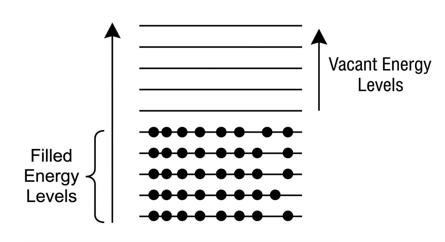
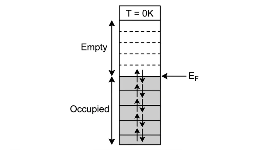
Fermi energy. The Fermi energy is the highest filled energy level at .
Case 2: at a finite temperature
When the solid is heated, some electrons are excited to higher levels. In a metal, is several electronvolts, while at room temperature . So .
- Electrons deep below cannot be excited, because the thermal energy is far too small to lift them to an empty level.
- Only electrons in a narrow band of width about just below can jump to levels just above .
As a result, the probability of finding electrons just below decreases below , and the probability of finding electrons just above increases above . The states above are partly occupied and the states just below are partly empty.
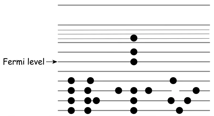
For an electron exactly at the Fermi level, , so the exponent is :
Key idea. At any temperature above , the probability of occupation of the Fermi level is , or 50 %. So the Fermi level can also be defined as the energy at which the occupation probability is one half.
Far from the Fermi level, not much changes:
- For , : high levels are still almost always empty.
- For , : low levels are still almost always full.
Case 3: at high temperature
As the temperature rises further:
- the electrons have more thermal energy and spread over a wider range of levels;
- the change from to becomes more and more gradual;
- a larger fraction of electrons occupies states above , and the probability of finding electrons just below falls further.
Far above the Fermi level, where , the in the denominator can be neglected:
This is the classical Maxwell–Boltzmann form. So at very high temperatures (or high energies), the Fermi–Dirac distribution starts to look like the classical one.
Graphical representation
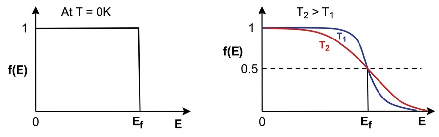
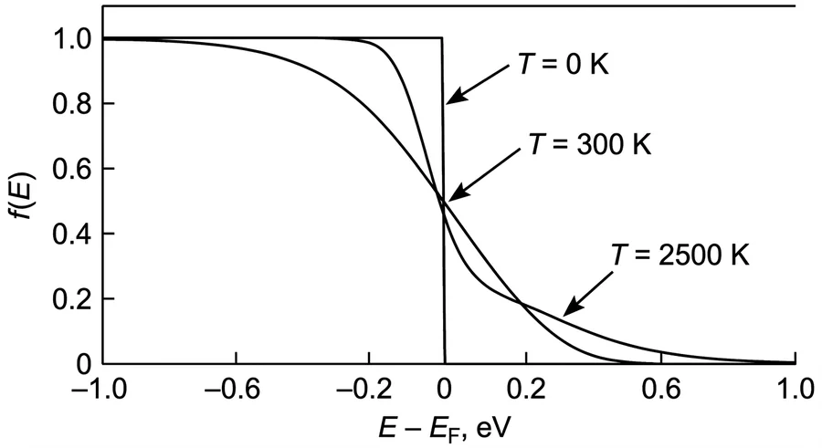
- At : a step. up to , and then a sudden drop to .
- At : the step becomes a smooth curve that falls from to over a width of a few around .
- At higher temperatures: the curve spreads out more and its tail looks like an exponential decay.
Every curve passes through at .
Watch out. At exactly , is indeterminate. Only for is . Examiners like this difference.
Page 11 of 25
The Fermi energy and Fermi level
Two definitions
- Fermi energy : the energy of the highest occupied level at .
- Fermi level: the more general term used at any temperature. It is the energy level whose probability of occupation is (50 %).
At absolute zero the two are the same. Many books use the two names in the same meaning.
Value of the Fermi energy
For a three-dimensional gas of free electrons, such as the conduction electrons of a metal, the Fermi energy is
where is the reduced Planck constant, is the electron mass and is the free electron density. It depends only on : the more electrons are packed in, the higher the levels they must fill.
From the Fermi energy we can also define the Fermi speed, the speed of an electron at the Fermi level:
Example 1. Copper has . Find its Fermi energy and Fermi speed.
With a relaxation time of , the mean free path at the Fermi speed is , about or more than 100 atomic spacings. This long mean free path is exactly what the classical theory could not explain.
Position of the Fermi level in different materials
Conductors (metals). The Fermi level lies inside the conduction band, or in the region where the conduction and valence bands overlap. Even at absolute zero there are free electrons in the conduction band, so metals conduct easily.
Semiconductors. The Fermi level lies within the band gap, between the valence and conduction bands. Its exact position depends on the type:
- in an intrinsic (pure) semiconductor it is near the middle of the gap;
- in an n-type semiconductor (doped with extra electrons) it moves closer to the conduction band;
- in a p-type semiconductor (doped with holes, or electron acceptors) it moves closer to the valence band.
Insulators. The Fermi level is also in the band gap, but the gap is much wider, so the Fermi level is far from both bands. It is extremely difficult for electrons to cross to the conduction band, so insulators have very few free electrons and do not conduct.
Watch out. "Fermi energy" strictly means the highest filled level at . "Fermi level" is the level at any temperature. Write which definition you are using. Also, in metals. Because of this, only a thin slice of electrons near takes part in conduction and heat capacity.
Page 12 of 25
Band theory: how energy bands form
Why a new theory
The free electron theories ignore the ion lattice. Band theory keeps the quantum picture but includes the effect of the crystal.
Basic assumptions
- Electrons have a wave nature, and the laws of quantum mechanics apply to them.
- The potential energy of an electron inside the crystal is not constant. It is lowest at the positive ion sites and highest midway between two ions, and this pattern repeats with the periodicity of the crystal.
Formation of energy bands
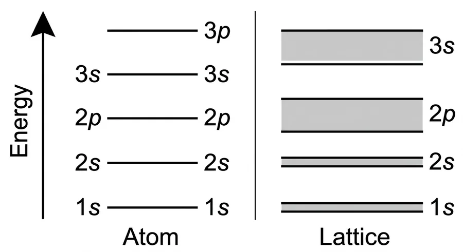
In a single, isolated atom, electrons occupy discrete energy levels, such as 1s, 2s, 2p, 3s, 3p.
When a very large number of atoms come close together to form a solid, the electron wave functions of neighbouring atoms overlap. Because of this interaction, and because the Pauli principle does not allow two electrons in a system to share the same state, each discrete atomic level splits into closely spaced levels. Together, these closely spaced levels form a continuous energy band.
Narrow and wide bands
- The electrons in the outer shells screen the inner (core) electrons from the neighbouring atoms. So the inner levels split only slightly and form narrow bands.
- The valence electrons in the outermost shell interact most strongly, so their levels split the most and form wider bands.
How close are the levels inside a band?
The width of an energy band is typically a few electronvolts. A crystal has an enormous number of atoms ( in a small piece), so the band has an enormous number of levels. So the energy gap between neighbouring levels is extremely small, of the order of
At room temperature, the thermal energy of an electron is about , which is much larger than this spacing. So inside an allowed band, an electron can easily move to a higher vacant level, either by thermal energy or under a small applied field. In effect, the levels in a band form a continuum.
Note on the source. The lecture notes gave the level spacing as about . If we divide a band of a few eV among about levels, we get about . In both cases the conclusion is the same: the spacing is negligible compared with .
Allowed and forbidden energies
Between the allowed bands there are ranges of energy in which no electron states exist. These are the forbidden bands or band gaps. An electron in a crystal can have an energy inside an allowed band, but never inside a gap. The next page looks at the two bands that decide the electrical behaviour.
Watch out. A band is made of levels, not of electrons. A band can be full, partly full or empty, depending on how many electrons are there to fill it.
Page 13 of 25
Valence band, conduction band and band gap
The energy band diagram
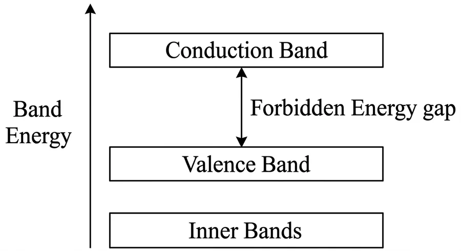
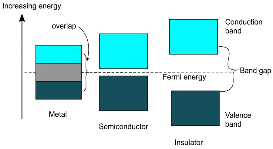
An energy band diagram shows the energy levels of the top energy band and the next lower band in a solid, with the gap between them. The vertical axis is electron energy. Bands are drawn as horizontal strips, with the inner bands at the bottom.
The two important bands
Valence band. The range of energies of the valence electrons that take part in bonding in the crystal. These electrons are bound to their atoms and are not free to move. The valence band is usually full or nearly full, so it cannot conduct well. Its top edge is , the highest energy an electron can have while still bound.
Conduction band. The range of higher energies of electrons that have broken free from their bonds and can move through the whole solid. Only free electrons take part in conduction, hence the name. Its bottom edge is , the smallest energy an electron must have to become free. An electron that reaches is no longer bound to an atom and can move under the effect of an electric field.
Forbidden band (band gap). The two bands are separated by a range of energies where no states exist. Its width is the band gap:
For an electron to take part in conduction, it must gain at least the energy to jump from , the top of the valence band, to , the bottom of the conduction band.
The band gap decides the behaviour
- If the bands overlap (no gap), electrons move freely between them. The material conducts easily.
- If the gap is moderate, electrons can be lifted across it by heat or light. This is a semiconductor.
- If the gap is large, electrons cannot cross it under normal conditions. This is an insulator.
Holes
When an electron leaves the valence band, it leaves behind an empty state, called a hole. A hole behaves like a positive charge carrier. Electrons in the valence band can move into the hole, so the hole effectively moves in the opposite direction. In a semiconductor, both the electrons in the conduction band and the holes in the valence band carry current.
Watch out. is the bottom of the conduction band and is the top of the valence band. The gap is measured between exactly these edges, not between the middles of the bands.
Page 14 of 25
Conductors, semiconductors and insulators
Conductors
Conductors are materials that allow current to flow easily.
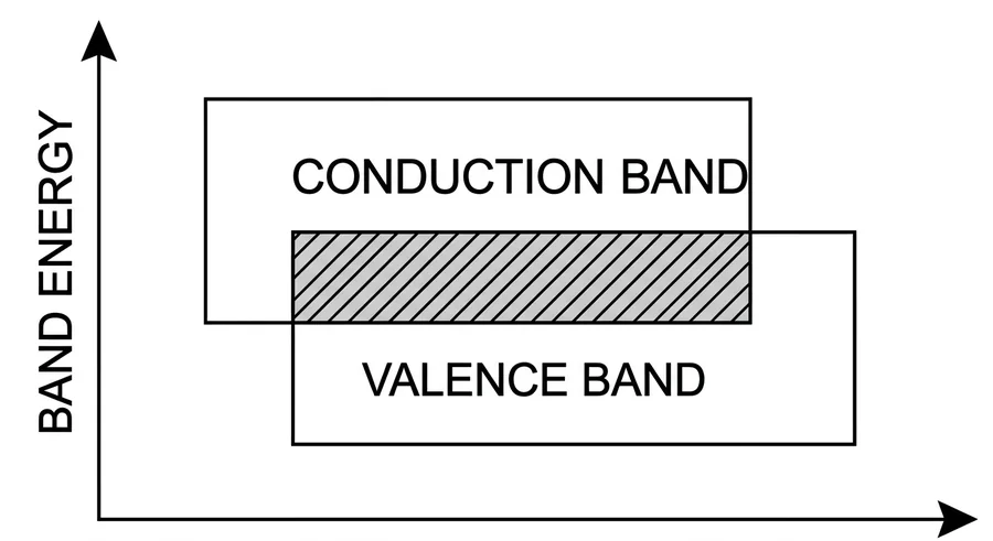
- The valence and conduction bands overlap, or the gap is negligible (less than about ).
- There is no significant energy barrier to stop electrons from entering the conduction band. Many electrons are already in it, and they move freely under an applied field.
- Even at room temperature there are plenty of free electrons, so metals are excellent conductors, and no extra energy is needed to excite electrons.
- The Fermi level lies inside the band.
- Examples: copper, silver, gold, aluminium, iron.
Semiconductors
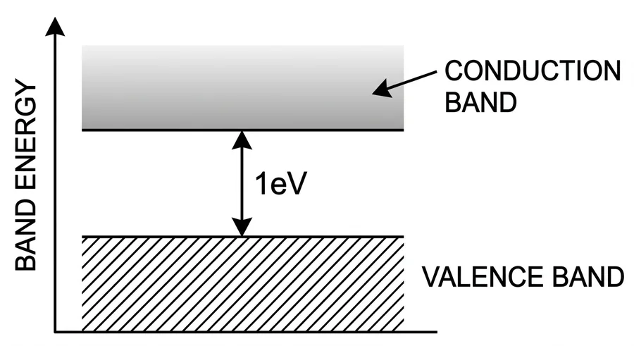
Semiconductors have a small but important band gap, roughly .
- At absolute zero the conduction band is empty and the valence band is full, with all electrons bound. So a semiconductor behaves as an insulator at .
- At room temperature, or when exposed to heat or light, some electrons get enough energy to cross the gap into the conduction band. Each one leaves a hole in the valence band.
- Both the free electrons and the holes carry current. Conduction is weaker than in a conductor because far fewer electrons are in the conduction band.
- Conductivity increases with temperature, so semiconductors have a negative temperature coefficient of resistance.
- Doping, which means adding small controlled amounts of impurity, can increase the conductivity enormously. Doping can increase the number of free electrons (n-type) or the number of holes (p-type). Because we can control this, semiconductors are very useful in electronic devices.
- Examples: silicon (), germanium (), gallium arsenide ().
Insulators
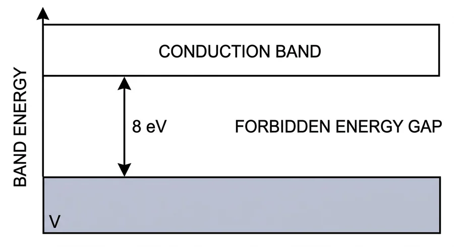
Insulators have a large band gap, roughly or more.
- Electrons in the valence band cannot get enough energy under normal conditions to jump across the gap, so there are very few or no electrons in the conduction band.
- Even an applied field cannot give enough energy to lift electrons across the gap. Conductivity is extremely poor because there are no free carriers.
- Only at very high temperatures do a few valence electrons reach the conduction band. Then the resistivity falls, so insulators also have a negative temperature coefficient of resistance.
- Because they have no free carriers, they are ideal for stopping the flow of current, for example to cover and enclose electrical wiring.
- Examples: diamond (), glass, rubber, wood, plastic.
Summary
| Conductor | Semiconductor | Insulator | |
|---|---|---|---|
| Band gap | overlap, or less than about | about | about or more |
| At | partly filled band, conducts | valence full, conduction empty: insulator | valence full, conduction empty |
| Effect of heating | resistance rises | conductivity rises sharply | conductivity rises only at very high |
| Temperature coefficient of resistance | positive | negative | negative |
| Fermi level | inside a band | in the gap | in the gap, far from both bands |
| Examples | Cu, Ag, Au, Al, Fe | Si, Ge, GaAs | diamond, glass, rubber |
Note on the source. The two lecture sets gave slightly different gap ranges: "1 to 2 eV" or "about 1 eV" for semiconductors, and "greater than 5 eV" for insulators. These are rough values, not sharp limits. The dividing line between a wide-gap semiconductor and an insulator is a matter of convention (around 3 to 4 eV). The values above are the usual textbook figures.
Page 15 of 25
Numerical problems: conductivity
Constants: , , .
Problem 1. A material has conductivity , carrier concentration and carrier effective mass . Find the relaxation time.
Step 1: effective mass. .
Step 2: rearrange to get .
Step 3: put the values. , so the denominator is , and the numerator is .
Problem 2. A metal has electron concentration and relaxation time . Find its conductivity.
Numerator: . Multiply the numbers, , and add the powers of ten, , to get .
so , close to the measured value for copper.
Problem 3. Find the drift velocity of the free electrons in a copper wire of cross-section carrying . Copper has density and atomic weight , and each atom gives one free electron.
Step 1: electron density. The number of atoms per unit volume is (density × Avogadro's number) / molar mass, with the molar mass in kg/mol:
Step 2: drift velocity from :
Even at the electrons drift less than a millimetre per second.
Problem 4. Find the mobility of electrons in copper, with valence electrons per and conductivity .
Problem 5. Find the relaxation time of conduction electrons in a metal of resistivity with conduction electrons per .
From :
Note on the source. The problem sheet printed the resistivity as , which would give . The answer given () needs , which is a typical value for a metal, so we have used that.
Problem 6. Silver has density and atomic weight , with one conduction electron per atom. Its conductivity at is . Find (a) the density of free electrons and (b) the electron mobility.
(a)
(b)
Problem 7. For the metal of Problem 2 carrying a current density of , find the field inside it and the drift velocity.
Watch out. Molar masses must be in kg/mol (), and areas in m². Most wrong answers on this page come from these two conversions.
Page 16 of 25
Numerical problems: the Fermi function and Fermi energy
Use when energies are in eV.
Problem 1. Find the probability that an electron occupies a state above the Fermi level at .
Step 1. .
Step 2. .
Step 3.
A state just above is almost empty at room temperature.
Problem 2. At what temperature is the probability of occupying a state above the Fermi level equal to ?
Step 1: rearrange. With ,
Step 2: take logs. .
Step 3: solve for .
Problem 3. At , find the probability that a state below the Fermi level is occupied, and that one above it is occupied.
.
They add up to . The chance of finding a hole below is equal to the chance of finding an electron above it.
Problem 4. Find the Fermi energy and Fermi speed of copper, .
is about 270 times at room temperature, which justifies treating only electrons near as active.
Problem 5. At what energy above is the occupation probability at ?
So the Fermi function falls from to within about of at room temperature. The "rounded step" is only a few wide.
Watch out. Use in eV/K when energies are in eV, and in J/K when they are in joules. Also remember that is a probability. Any answer above or below is wrong.
Page 17 of 25
Superconductivity: discovery and transition temperature
What superconductivity is
Superconductivity is a phenomenon in which some materials, when cooled below a certain temperature, show two special properties:
- zero electrical resistance, and
- expulsion of magnetic fields from their inside.
The temperature below which this happens is called the critical temperature or transition temperature, .
Discovery
- Superconductivity was discovered in 1911 by the Dutch physicist Heike Kamerlingh Onnes, who was studying the electrical resistance of mercury at very low temperatures.
- He found that at about 4.2 K the resistance of mercury suddenly dropped to zero. This was the start of superconductivity.
- A superconducting material conducts electric current without any loss of energy, which is very different from any ordinary conductor.
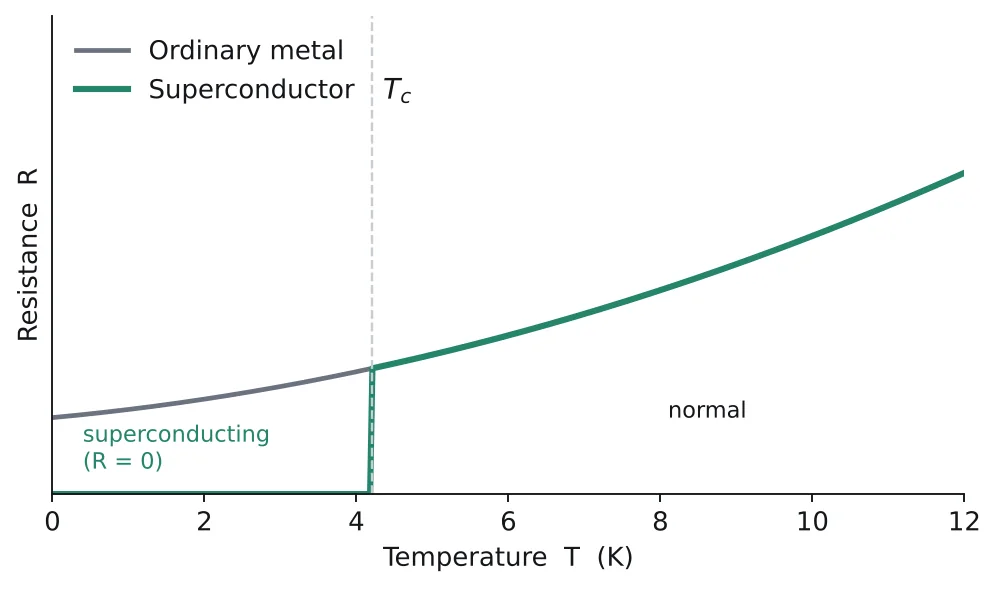
In an ordinary metal the resistance falls as it is cooled but becomes steady at a small finite value (because of impurities and defects). In a superconductor it falls suddenly to exactly zero at .
The transition (critical) temperature
Transition temperature . The temperature below which a material changes from the normal conducting state to the superconducting state.
- Above : the material behaves as a normal conductor, with finite resistance and no expulsion of the magnetic field.
- Below : the material is superconducting, with zero resistance and the Meissner effect.
- Each superconductor has its own , from near to above for the high-temperature superconductors.
- High-temperature superconductors, such as some ceramic materials, have above . They are easier to use in practice because they can be cooled with liquid nitrogen (which boils at ) instead of expensive liquid helium (which boils at ).
- The transition is reversible. If the material is warmed above , it goes back to the normal state, its finite resistance comes back, and any magnetic field that was pushed out enters it again.
Critical temperatures of some superconductors
| Material | Type | |
|---|---|---|
| Tin (Sn) | I | |
| Mercury (Hg) | I | |
| Lead (Pb) | I | |
| Niobium (Nb) | II | |
| Magnesium diboride (MgB₂) | II | |
| Yttrium barium copper oxide (YBCO) | II |
History of the transition temperature
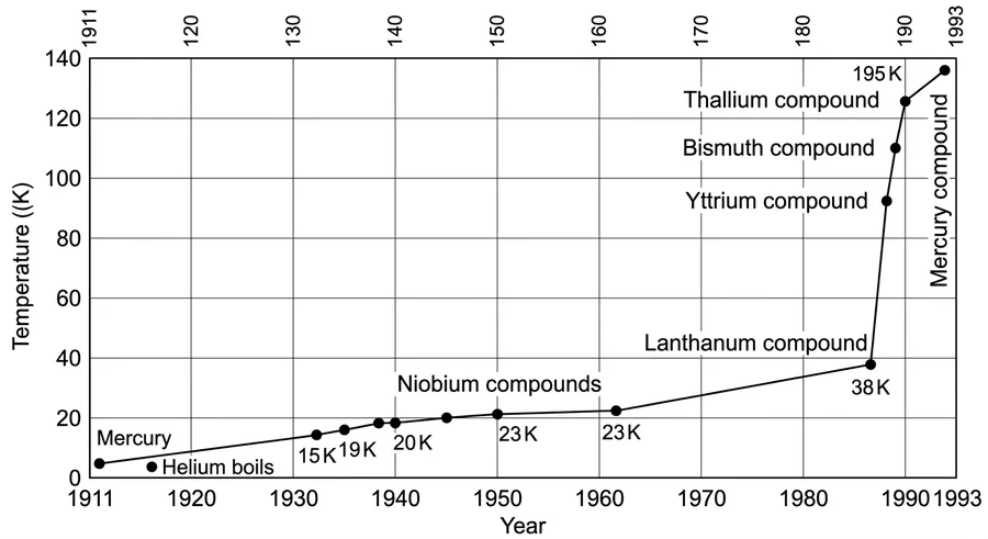
For 75 years after the discovery, the highest known increased slowly through niobium compounds to about . In 1986 the copper-oxide (cuprate) ceramics were discovered, and within a few years went above the boiling point of liquid nitrogen: about for yttrium compounds, over for bismuth and thallium compounds, and about for mercury compounds.
Watch out. Above a superconductor is just an ordinary conductor, often not a very good one. Lead, mercury and tin conduct worse than copper at room temperature.
Page 18 of 25
Properties of superconductors
Some facts about superconducting materials
- Apart from pure elements, many compounds and alloys are superconductors.
- Good conductors of current such as copper, silver and gold are not superconductors.
- Some elements become superconducting only under high pressure, and others only in special forms such as thin films.
- Compounds generally have higher transition temperatures than elements.
- A superconducting binary compound may be made from two superconducting elements, from one superconducting and one non-superconducting element, or even from two elements neither of which is a superconductor.
1. Zero resistance
Below the electrical resistance is exactly zero, so there are no losses. Most applications are based on this property.
2. Persistent currents
A persistent current is a steady current that flows without diminishing in strength.
- Once such a current is set up in a closed superconducting loop, no external power supply is needed to keep it going, because there are no losses.
- As long as the loop is kept below , the current keeps flowing without decay. Persistent currents have been seen to flow for years with no measurable decrease.
3. Flux quantisation
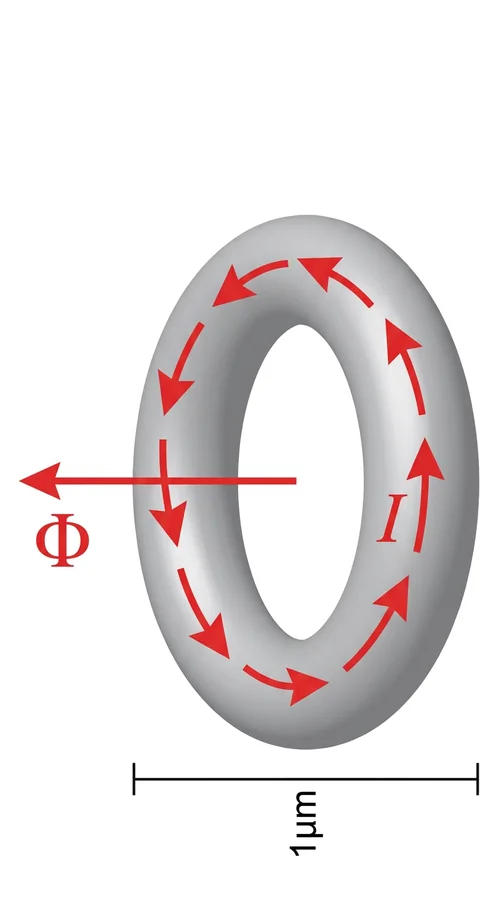
Consider a current flowing round a superconducting ring.
- The magnetic flux density inside the superconducting material itself is zero, but magnetic flux can exist in the hole in the middle of the ring.
- This flux cannot take any value. It can only be a whole-number multiple of a basic unit, the flux quantum or fluxon:
- Numerically,
This is flux quantisation. The charge in the denominator is the charge of a Cooper pair of electrons (see BCS theory), so flux quantisation is direct evidence that the current in a superconductor is carried by pairs.
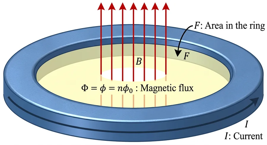
Example 1. A superconducting ring of area has a field of through it. How many flux quanta does it hold?
4. Isotope effect
The transition temperature depends on the mass of the ions. Heavier isotopes of the same element have a lower ,
This shows that the vibrations of the lattice take part in superconductivity, which is a key idea of BCS theory.
Example 2. Two isotopes of mercury have masses and . Find the ratio of their critical temperatures.
The heavier isotope has a about lower.
5. Effect of magnetic field and the Meissner effect
A strong enough magnetic field destroys superconductivity (the critical field), and a superconductor expels magnetic flux (the Meissner effect). These two properties are covered on the next pages, after a short review of magnetism.
| Property | Summary |
|---|---|
| Zero resistance | below |
| Persistent current | flows without decay in a closed loop |
| Flux quantisation | through a ring |
| Isotope effect | |
| Critical field | strong field destroys superconductivity |
| Meissner effect | inside, |
Watch out. "Zero resistance" alone would describe a perfect conductor. What makes a superconductor a really new state is that it also expels magnetic fields.
Page 19 of 25
Review of magnetism
The Meissner effect and the critical field use a few magnetic quantities. Here they are in one place.
- Magnetic field. The region of space around a magnet, a current-carrying conductor or a moving charge, in which a magnetic effect can be felt, is called a magnetic field.
- Magnetic induction . If a field is strong, its field lines are closer together. The magnetic induction or magnetic flux density at a point is the flux (number of field lines) passing through unit area around that point. Its unit is the tesla (T).
- Magnetising field . The field due to currents in external circuits (for example a solenoid) is called the magnetising field . Its SI unit is ampere per metre (A/m).
- Magnetisation . When a material is placed in a magnetic field, it becomes magnetised. The magnetic moment per unit volume of the material is its intensity of magnetisation . It tells how much the specimen is magnetised. Its unit is also A/m.
- Permeability . The magnetic permeability of a material is the ratio of the resultant field inside the material to the magnetising field :
Its unit is henry per metre (H/m). The permeability of free space is a constant, .
- Susceptibility . The ratio of magnetisation to magnetising field is the magnetic susceptibility:
It has no unit.
- Permeability versus susceptibility. Permeability tells how well a material supports the formation of a magnetic field inside itself. Susceptibility tells whether the material is attracted to a magnetic field or repelled from it.
- Sign of . is negative for diamagnetic substances (weakly repelled) and positive for paramagnetic substances (weakly attracted).
- The connecting relation. Magnetisation , magnetising field and magnetic induction are related by
Summary
| Quantity | Meaning | Unit |
|---|---|---|
| magnetic flux density | T | |
| magnetising field | A/m | |
| magnetic moment per unit volume | A/m | |
| permeability | H/m | |
| susceptibility | none |
Watch out. and have the same unit (A/m), so has no dimension. Do not write a unit for in an exam answer.
Page 20 of 25
Critical field
The idea
A superconductor stays superconducting only if the magnetic field applied to it is not too strong.
Critical field . The maximum magnetic field strength that a superconductor can bear while remaining in the superconducting state. If the applied field is more than , superconductivity is destroyed and the material goes back to the normal state with finite resistance.
Variation with temperature
- The critical field depends on temperature. It is largest at and decreases as the temperature comes close to , where it becomes zero.
- The variation is well described by
where is the critical field at .
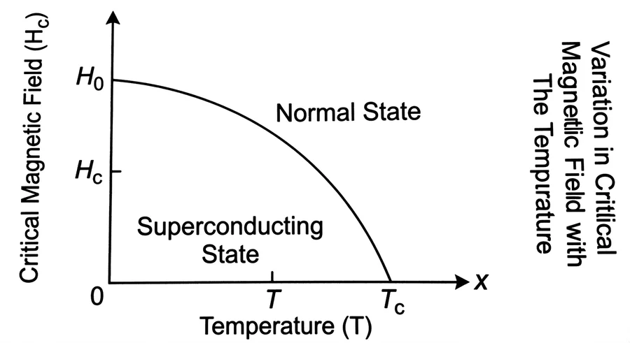
The curve divides the – plane into two regions. Any combination of field and temperature below the curve is superconducting. Any combination above it is normal. To destroy superconductivity you can raise the temperature above , or raise the field above , or do a bit of both.
Why it matters
The critical field is an important parameter for applications. Superconducting magnets in MRI machines and particle accelerators must stay superconducting while producing very strong fields, so they need materials with high critical fields. Superconductors with higher critical fields can work in stronger magnetic fields without losing their superconducting properties.
Examples
Example 1. Lead has and . Find its critical field at .
Example 2. At what fraction of is the critical field half its value at ?
More examples are on the practice page.
Watch out. The temperature ratio is squared in the formula. Also, is zero at , not at . The field a superconductor can bear is greatest when it is coldest.
Page 21 of 25
The Meissner effect
The idea
Meissner effect. When a superconducting material is cooled below its critical temperature in a magnetic field, it expels all the magnetic field lines from its inside. The magnetic flux density inside becomes zero, .
The Meissner effect is one of the defining characteristics of superconductivity. It was discovered by Walther Meissner and Robert Ochsenfeld in 1933.
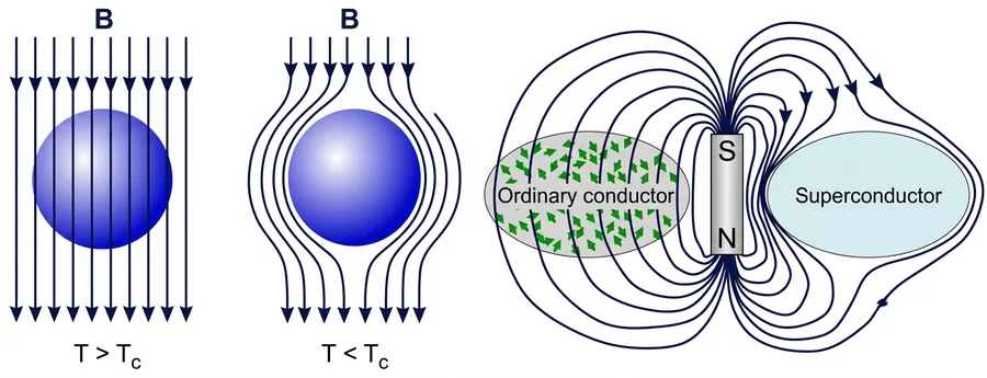
- Above : the field lines pass straight through the material.
- Below : the field lines bend around the material and none enter it.
- An ordinary conductor near a magnet lets the field pass through it. A superconductor pushes the field out completely.
Superconductor versus perfect conductor
A hypothetical "perfect conductor" with zero resistance would simply freeze in whatever field was inside it when it lost its resistance: if it was cooled in a field, the field would stay trapped inside. A superconductor behaves differently. It actively expels the field, whether the field was applied before or after cooling. This is why superconductivity is a genuinely new state of matter, not just very good conduction.
Proof that a superconductor is a perfect diamagnet
For any material, the magnetic induction is related to the magnetising field and magnetisation by
In a superconductor, by the Meissner effect, the total field inside is zero:
Put this in:
Since ,
So the magnetic susceptibility is
Key idea. is the condition for perfect diamagnetism. The Meissner effect makes a superconductor a perfect diamagnet. No ordinary material has this property. Ordinary diamagnets have of only about .
Consequences
- A small magnet placed above a superconductor is repelled and can levitate, floating above the surface. This is the basis of magnetic levitation.
- Because the material repels the field, there is a sharp change in the magnetic behaviour at , which can be used to detect the transition.
Watch out. The Meissner effect means inside the material. The applied field is not zero. It is cancelled by the magnetisation . Also, is true only for the complete Meissner state: Type I below , or Type II below .
Page 22 of 25
Type I and Type II superconductors
Superconductors are divided into two types according to how they respond to an increasing applied magnetic field.
Type I superconductors
- Type I superconductors show superconductivity and completely expel magnetic fields below a critical temperature and a critical field .
- They show the complete Meissner effect. Below they are perfectly diamagnetic and the flux is totally expelled ().
- They are usually pure elements.
- They have only one critical field, .
- At the transition to the normal state happens sharply. The magnetisation drops suddenly to zero and the magnetic lines of force suddenly enter the material.
- There is no mixed state.
- Their critical field is usually low, so only a small field is needed to destroy superconductivity. So they are called soft superconductors, and they are limited to low-field applications.
- Examples: lead (), mercury (), tin ().
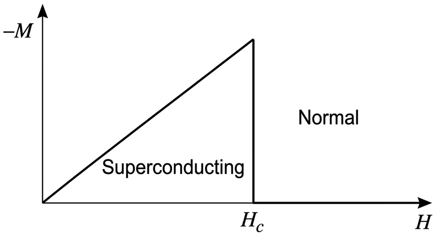
The magnetisation graph rises linearly (perfect diamagnetism, ) up to and then drops vertically to zero. The resistance shows the same sudden change: it is zero up to , and then jumps to its normal value.
Type II superconductors
- Type II superconductors allow magnetic fields to partly enter while staying superconducting.
- They show a partial Meissner effect.
- They include pure elements as well as alloys and compounds.
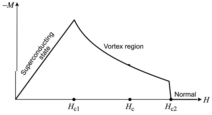
- They have two critical fields, a lower critical field and an upper critical field .
- Below : the material is perfectly diamagnetic, with the flux totally expelled (), as in the complete Meissner effect.
- At : magnetic field lines start to enter the material in small amounts.
- Between and : the material is still diamagnetic, but not perfectly (), so the Meissner effect is incomplete. Magnetic flux enters as thin filaments called vortices, while the rest of the material stays superconducting. This is the mixed state or vortex state. Electrically the material is still a superconductor, but magnetically it is in a mixed state.
- At : the magnetisation becomes zero, the flux enters completely, and the material becomes a normal conductor. Above superconductivity is completely destroyed.
- The magnetisation is lost gradually, not suddenly.
- They usually have higher critical temperatures and much higher critical fields than Type I. Since a very large field is needed to destroy their superconductivity, they are called hard superconductors.
- This makes them useful for applications such as superconducting magnets and quantum computing.
- Examples: niobium (), yttrium barium copper oxide (), magnesium diboride ().
Comparison
| Type I (soft) | Type II (hard) | |
|---|---|---|
| Critical fields | one, | two, and |
| Meissner effect | complete below | complete below , partial between and |
| Mixed (vortex) state | absent | present between and |
| Loss of magnetisation | abrupt, at | gradual, from to |
| Size of critical field | low | high |
| Typical materials | pure elements | alloys, compounds, some elements |
| Uses | limited (low fields) | high-field magnets, MRI, accelerators |
| Examples | Pb, Hg, Sn | Nb, MgB₂, YBCO |
Watch out. In the Type II graph the magnetisation does not drop to zero at . It starts to fall there and reaches zero only at . Between the two fields the material still conducts without resistance.
Page 23 of 25
BCS theory of superconductivity
Background
The BCS theory is the microscopic theory of superconductivity, developed in 1957 by John Bardeen, Leon Cooper and Robert Schrieffer (hence BCS). It is based on quantum mechanics, and it won the three scientists the 1972 Nobel Prize in Physics "for their jointly developed theory of superconductivity". It explains how superconductivity arises at low temperatures and gives a framework for understanding superconductors.
The problem it solves
In the normal state, a conduction electron is repelled by other electrons and attracted by the positive ion cores. These forces act in random directions, and they scatter the electron as it moves through the material. This scattering is the cause of resistance.
According to BCS theory, below the critical temperature the conduction electrons form pairs that attract each other, and these pairs move without scattering. The pairing is due to an electron–lattice–electron interaction.
Formation of Cooper pairs
Normally two electrons, both being negatively charged, repel each other. At low temperatures they can attract each other through the lattice:
- Suppose two electrons, 1 and 2, pass each other in the crystal lattice.
- The negative charge of electron 1 attracts the positive ions of the lattice towards it, and slightly distorts the lattice.
- The extra positive charge collected around electron 1 screens its negative charge.
- Because of this screening, electron 2 is attracted towards the region around electron 1. The two electrons form a bound state.
- In terms of lattice vibrations: electron 1's interaction with the lattice emits a phonon (a quantum of lattice vibration), and electron 2 absorbs that phonon. The exchange of the phonon produces an attractive force between the two electrons.
This pair of electrons attracting each other is called a Cooper pair. Phonons act like the "glue" that holds the electrons together.
Key idea. The attraction is strongest when the two electrons have equal and opposite spins and opposite momenta. So a Cooper pair has zero total spin and, when no current flows, zero total momentum.
Why a Cooper pair has no resistance
- Energy gap. When electrons form Cooper pairs, an energy gap opens in the energy spectrum of the material. A certain minimum energy is needed to break a pair.
- Only below . Pairs form only below the critical temperature, because only then are the thermal vibrations of the lattice too weak to break them. Below the thermal energy is not enough to cross the energy gap.
- Coherent motion. All the Cooper pairs in a superconductor are in the same quantum state. They show phase coherence and move together as a single entity.
- No scattering. Cooper pairs are not scattered by the lattice points. Any disturbance would have to give at least the gap energy to break a pair, and below that energy is not available. So no energy is transferred from the electron pairs to the lattice.
- Zero resistance. If a field is applied, the pairs gain extra kinetic energy and give rise to a current, but they do not pass this energy to the lattice, so they are not slowed down. As a result, the material has no electrical resistance.
Evidence for the theory
- The isotope effect () shows that lattice vibrations, and hence phonons, are involved.
- Flux quantisation in units of shows that the charge carriers have charge . So they are pairs.
- The energy gap predicted by the theory is seen in experiments.
Limits of the theory
BCS theory explains conventional superconductors, the low-temperature metals and alloys in which phonons provide the pairing. It does not explain the high-temperature ceramic (cuprate) superconductors, whose mechanism is still being researched.
Note on the source. One lecture set said that BCS "explains only Type I superconductivity". The more correct statement is that BCS describes conventional (phonon-mediated, low-) superconductors, whether Type I or Type II, but not the high- ceramics.
Watch out. Electrons repel each other directly. The attraction in a Cooper pair is indirect, and it comes through the lattice. Do not write that "electrons attract each other at low temperature" without explaining that the lattice is the go-between.
Page 24 of 25
Applications of superconductors
Zero resistance, persistent currents, high critical fields and the expulsion of magnetic fields give superconductors many uses.
- Magnetic Resonance Imaging (MRI). Superconducting magnets produce the strong, stable magnetic fields needed in MRI machines. The high field strength gives better image resolution and clarity.
- Maglev trains. Magnetic levitation trains use superconducting magnets. The coaches do not slide on steel rails but float on a cushion of air (about 10 cm) above the track. This removes friction and the loss of energy as heat, so the trains can reach speeds of about , and travel faster, more smoothly and more efficiently.
- Particle accelerators. Superconducting magnets steer and focus particle beams at high energies, for example in the Large Hadron Collider (LHC).
- Quantum computing. Superconducting qubits are used in quantum computers. Their superconducting circuits can exist in superpositions of states, which allows new kinds of computation.
- Power transmission. Superconducting cables carry electricity without resistive losses. If a grid were made of superconducting wire, there would be no need to step up the voltage for transmission and step it down again, and the efficiency and reliability of the grid would improve greatly.
- Electrical machines. Motors, generators and transformers can be made smaller, lighter and much more efficient, with no eddy-current loss, hysteresis loss or resistive loss in the windings.
- SQUIDs. A Superconducting QUantum Interference Device is an extremely sensitive magnetometer. It can measure magnetic fields as weak as about . SQUIDs are used:
- by geologists, to measure rock magnetism and continental drift;
- in medicine, to measure muscular and neural activity (for example, the magnetic fields of the heart and brain);
- in non-destructive testing, for example to detect corrosion in aluminium sheets riveted together in aircraft.
- Energy storage (SMES). Superconducting Magnetic Energy Storage systems store energy in the magnetic field of a current circulating in a superconducting coil. They respond very fast and are highly efficient, so they are used to stabilise electrical grids and provide backup power.
- Electronic switches. Switching a superconductor between its normal and superconducting states (for example with a magnetic field) gives a fast switch, the cryotron.
- Telecommunications. Superconducting components reduce noise and improve signal quality in communication systems, especially in radio-frequency and high-frequency circuits.
| Property used | Applications |
|---|---|
| Zero resistance | power cables, motors and generators, energy storage |
| Strong, stable field (high ) | MRI, particle accelerators, maglev |
| Meissner effect (levitation) | maglev trains |
| Flux quantisation and quantum coherence | SQUIDs, qubits |
| Switching between states | cryotron switches |
Watch out. All these applications need cooling below , which is their main practical cost. That is why high-temperature superconductors, which can be cooled with cheap liquid nitrogen, are so attractive.
Page 25 of 25
Practice questions and formula sheet
Superconductivity numerical problems
1. The transition temperature of lead is . At it loses its superconductivity in a field of . Find the maximum field at which lead stays superconducting at .
2. The critical field of niobium is at and at . Find its transition temperature.
3. The transition temperature of lead is and its maximum critical field is . It is to be used in a field of . What precaution is needed?
The lead must be kept below . Above that, the field of destroys its superconductivity.
4. For a superconducting isotope of mass the critical temperature is . Find the isotopic mass for which it is .
Note on the source. The lecture sheet gave . When the ratio is calculated exactly, we get . The difference is due to rounding in the source.
Quick practice (answers at the end)
- A metal has and . Find and .
- Find for a state above at .
- Find the critical field of mercury (, ) at .
- What is the magnetic susceptibility of a superconductor in the Meissner state, and what is inside it?
Answers. (5) , . (6) , so . (7) . (8) and .
Exam-style questions to revise
- Define drift velocity, relaxation time, mean free path and mobility. Give their units.
- List the assumptions of the classical free electron theory.
- Derive an expression for the electrical conductivity of a metal on the basis of the classical free electron theory. Define mobility and relate it to conductivity.
- What are the factors affecting the conductivity of metals?
- Give the drawbacks of the classical free electron theory. How does the quantum free electron theory overcome them?
- State the Fermi–Dirac distribution function. Discuss its variation with temperature, with graphs.
- Define Fermi energy. Show that the probability of occupancy of the Fermi level is at any temperature above .
- Explain the formation of energy bands in solids. Classify materials into conductors, semiconductors and insulators on the basis of band theory.
- What is superconductivity? Define transition temperature and critical field. How does the critical field vary with temperature?
- Explain the Meissner effect and show that a superconductor is a perfect diamagnet.
- Distinguish between Type I and Type II superconductors, with magnetisation curves.
- Explain the BCS theory of superconductivity. What is a Cooper pair?
- What are persistent currents and flux quantisation?
- Describe the applications of superconductors.
Formula sheet
Conductivity
| Resistivity | , |
| Point form of Ohm's law | |
| Drift velocity | (in magnitude) |
| Current density | , |
| Conductivity | |
| Mobility | |
| Mean free path | |
| Electron density | (one free electron per atom) |
| Wiedemann–Franz | , |
Fermi–Dirac and bands
| Distribution | |
| At | for , for |
| At | |
| Symmetry | |
| High energy limit | |
| Fermi energy | |
| Fermi speed | |
| Band gap | |
| Constants |
Superconductivity
| Critical field | |
| Field relation | , , |
| Meissner state | |
| Flux quantum | , |
| Isotope effect |