
Page 1 of 15
Module 2 at a glance
Quantum mechanics is the branch of mechanics that gives the mathematical description of the motion and interaction of very small particles such as electrons, protons and atoms. Classical (Newtonian) mechanics works perfectly for cricket balls and planets, but it fails at the atomic scale. It cannot explain why atoms are stable, why their spectra have sharp lines, or why electrons are diffracted by crystals. Quantum mechanics takes its place there. It is based on three ideas that have no place in everyday physics:
- Quantisation of energy. A confined particle cannot have any energy it likes. Only certain discrete energies are allowed.
- Wave–particle duality. Every moving particle has a wave associated with it, called the matter wave. The wave is described by a wave function , and tells where the particle is likely to be, not where it definitely is.
- The uncertainty principle. Position and momentum (and also energy and time) cannot both be known exactly at the same time.
From these ideas we build the Schrödinger equation, the equation that the wave function follows. We solve it for two standard problems: a particle trapped in a box (which explains why energy comes in discrete levels and why a confined particle can never be at rest) and a particle meeting a barrier that it does not have enough energy to climb (which explains tunnelling).
What you will be able to do
- Derive the de Broglie relation and calculate the wavelength of any particle, and of an electron accelerated through a voltage.
- Explain the physical meaning of the wave function (Born's interpretation), write the conditions for a well-behaved wave function, and normalise a wave function.
- Write the wave function of a free particle and show that and .
- Explain wave packets, phase and group velocity, and how a wave packet leads to the uncertainty principle.
- State the uncertainty principle for the three conjugate pairs and use it to show that electrons cannot exist inside the nucleus and that spectral lines have a natural width.
- Derive the time-dependent Schrödinger equation by two methods, and derive the time-independent equation from it.
- Solve the Schrödinger equation for a particle in a one-dimensional box: find the energy eigenvalues and the normalised eigenfunctions, and interpret them.
- Explain quantum mechanical tunnelling, write the wave function in each region, define the transmission coefficient and list its applications.
How to use these notes
- Each page follows idea → explanation or derivation → worked example → common mistakes.
- Green boxes show key ideas and definitions. Amber boxes marked Watch out show mistakes that make you lose marks. Boxes marked Note on the source show where the lecture notes were corrected.
- The derivations of the Schrödinger equation and the particle in a box are the most frequently asked essay questions. Read them, then close the notes and write them yourself, step by step, until you can do it without looking.
- The last page has practice problems with full answers, the past KTU exam questions and a formula sheet.
Where each topic sits
| Part | Pages |
|---|---|
| Matter waves | Matter waves, de Broglie wavelength examples |
| The wave function | Wave function and probability, normalisation, the free-particle wave function, wave packets |
| Uncertainty | Uncertainty principle, its applications |
| Schrödinger equation | Time-dependent form (two derivations), time-independent form |
| Applications | Particle in a box (solution, then energies and wave functions), tunnelling |
| Revision | Practice questions, exam questions and formula sheet |
Before you start. You should know wavelength , frequency , period , angular frequency and wave number ; the photon relations and ; complex numbers, with , the conjugate and ; partial derivatives and simple integration, including .
Page 2 of 15
Matter waves
The idea
By the early twentieth century it was clear that light has a dual nature. Interference, diffraction and polarisation show that light is a wave. The photoelectric effect and the Compton effect show that light also behaves as a stream of particles, called photons, each carrying energy and momentum .
In 1924 the French physicist Louis de Broglie argued by analogy and symmetry: if waves (light) can behave like particles, then particles should also be able to behave like waves. He proposed that every moving object has a wave associated with it under suitable conditions. These waves are called matter waves or de Broglie waves.
Matter waves. The waves associated with a moving particle are called matter waves or de Broglie waves. Their wavelength is called the de Broglie wavelength.
Deriving the de Broglie wavelength (route 1: from the photon's energy)
For a photon the energy can be written in two ways, one from its wave nature and one from its particle nature:
Since both describe the same photon, they must be equal. This shows its wave–particle dual nature:
Cancel one factor of :
Here (mass times velocity) is the momentum of the photon. So
Deriving it (route 2: from the photon's momentum)
The momentum of a photon is known directly from experiment and theory to be , which can be written as . De Broglie's step was to assume that this equation is completely general. It applies not only to photons but to electrons, protons, atoms and every other particle.
The de Broglie wavelength of a particle
A particle of mass moving with speed has momentum . Its kinetic energy is , which can be written as
so the de Broglie wavelength can be written in three equivalent ways:
de Broglie wavelength.
An electron accelerated through a voltage
An electron of charge and mass , starting from rest and accelerated through a potential difference of volts, gains kinetic energy . So
Then the wavelength of the electron is
This is the same as putting in . Now put , and :
Since , the same result in ångström is
(because ). Both forms appear in textbooks; they are the same formula.
Watch out. These shortcut formulas are only for electrons, because the mass and charge of the electron are already inside the number . For a proton, neutron, alpha particle or anything else, go back to with the correct mass.
Some properties of matter waves
- The lighter the particle, the longer its wavelength for a given speed (). This is why wave effects are noticeable for electrons but not for everyday objects.
- The faster the particle, the shorter its wavelength ().
- A particle at rest () would have an infinite wavelength. Matter waves are associated only with moving particles.
- Matter waves are not electromagnetic waves. They are produced by any moving particle, charged or neutral (neutrons are also diffracted).
- The wave is not a physical disturbance of a medium. As the wave function pages explain, it is a probability wave.
Experimental evidence
De Broglie had no experimental evidence when he proposed the idea. But he could show that it explained the stationary orbits and the quantised energy levels that Bohr had assumed for the hydrogen atom in 1913. An electron orbit is allowed only if a whole number of de Broglie wavelengths fits around it, , which is exactly Bohr's condition on angular momentum.
The direct proof came in 1927. Davisson and Germer in the USA, and independently G. P. Thomson in Britain, showed that electrons are diffracted by crystals exactly as X-rays are, with the wavelength given by . Today, electron diffraction and the electron microscope depend on this.
Key idea. Wave and particle are two aspects of the same object. Which aspect we see depends on the experiment. Diffraction shows the wave, and a collision with a detector shows the particle.
Page 3 of 15
de Broglie wavelength: worked examples
Constants: , , , , .
Example 1. Why we never notice matter waves. Find the de Broglie wavelength of (a) a ball of mass moving at , and (b) an electron accelerated through .
(a) First convert the speed: . Then
This is roughly , which is extremely small compared with the size of the ball (and far smaller than even a nucleus). No experiment can ever detect a wave aspect in the behaviour of the ball, so for everyday objects classical mechanics is perfectly good.
(b) Using the electron formula,
This is about the size of an atom, and it is much larger than the classical radius of the electron (). So the wave nature of the electron cannot be neglected. It is also comparable to the spacing between atoms in a crystal, which is why crystals diffract electrons.
Note on the source. One lecture set gave the wavelength of the electron in part (b) as . The correct value is , ten times larger, as the formula shows for .
Example 2. The Davisson–Germer experiment. In the original experiment the electrons were accelerated through . Find their wavelength.
This matched the wavelength measured from the diffraction pattern of a nickel crystal, and this is how the experiment confirmed de Broglie's hypothesis.
Example 3. A slow (thermal) neutron. Find the de Broglie wavelength of a neutron with kinetic energy .
The electron formula cannot be used. Change the energy to joules, , and use the general form:
Again about . Slow neutrons are diffracted by crystals and are used to study crystal structures.
Example 4. A proton versus an electron. A proton and an electron are each accelerated through . Compare their wavelengths.
Both gain the same kinetic energy , so :
The proton's wavelength is about 43 times shorter, because it is 1836 times heavier.
Example 5. Reverse problem. Through what voltage must an electron be accelerated to have a wavelength of ?
From : , so .
Watch out. Always work in SI units: mass in kg (500 g is kg), speed in m/s (divide km/h by 3.6) and energy in joules (multiply eV by ). Most wrong answers here come from a unit that was not converted.
Page 4 of 15
The wave function and probability
The idea
In every wave, something varies periodically with space and time:
| Wave | What varies |
|---|---|
| Water wave | the height of the water surface |
| Sound wave | the pressure of the air |
| Light (electromagnetic) wave | the electric and magnetic fields |
| Matter wave | the wave function |
The quantity whose variations make up matter waves is called the wave function, written (the Greek capital letter psi, pronounced "sigh"). In general it is a function of all three space coordinates and of time:
The wave function is a mathematical function that represents the state of the particle. The mathematical theory of quantum mechanics tells how to use to find the position, velocity, momentum, energy, angular momentum and so on of the particle. Everything that can be known about the particle is contained in .
Physical significance (Born's interpretation)
- itself cannot be measured. The wave function is in general a complex quantity (it contains ). A complex number cannot be the result of a measurement, so has no direct physical meaning by itself.
- is real and measurable. The square of the absolute value of ,
where is the complex conjugate of , is always real and positive.
- is a probability density. represents the probability of finding the particle at the point at time , per unit volume. It is called the probability density or the probability distribution function. Where is large, the particle is likely to be found. Where it is small, the particle is unlikely to be found.
- Probability in a region. The probability of finding the particle in a small volume around at time is . For a finite region it is the integral
always lies between (never there) and (certainly there). For example, if for a region, there is a 40 % chance of finding the particle in that region.
- Probability amplitude. itself is not a probability, but its square is. So is also called the probability amplitude.
- Statistical link between wave and particle. The wave function connects the particle nature and the wave nature statistically. It does not tell exactly where the particle is. It tells where the particle is likely to be. If we repeat the same experiment many times, the particle is found most often where is largest.
Key idea. Quantum mechanics does not predict the exact location of a particle. It predicts the probability of finding it in each region of space. The matter wave is a probability wave.
A one-dimensional picture
For a particle moving only along , the wave function is and is the probability of finding the particle between and . The probability of finding it between and is
Watch out. The probability density is , not . For a complex , is itself complex and cannot be a probability. Only when is real (as for the particle in a box) are the two the same.
Page 5 of 15
Normalisation and well-behaved wave functions
Normalisation
A particle that exists in a particular region must be found somewhere in that region. So the probability of finding it anywhere in the region must be exactly 1 (100 %):
A wave function that satisfies this is said to be normalised (normalised to unity).
Now suppose we have a wave function that solves the Schrödinger equation but is not normalised. If we multiply a solution by a constant (not depending on , , ), we get another solution, . We choose so that the new wave function is normalised. Adding the probability at all points in the volume ,
Normalisation. The process of multiplying a wave function by a suitable constant so that the probability of finding the particle within the region becomes exactly 1 is called normalisation. The constant is called the normalisation constant.
Why a wave function must be normalisable
is supposed to be a probability density. A probability can only be interpreted if the total adds up to 1, so the integral must be finite. A wave function whose integral is infinite cannot be normalised and cannot describe a real particle.
Conditions for a well-behaved wave function
The physically acceptable ("well-behaved") wave functions satisfy these conditions:
- is finite everywhere. An infinite value would mean an infinite probability.
- is single-valued. At any point and time there must be only one value of the probability.
- is continuous. The probability cannot jump suddenly from place to place.
- The first derivatives , , are continuous and single-valued, wherever the potential is finite. These derivatives decide the momentum of the particle, which must change smoothly.
- is normalisable, so as .
Worked example
Example 1. A particle confined between and has the wave function inside, and outside. Find the normalisation constant .
Normalisation requires
Expand and integrate term by term:
So , giving
This function is finite, single-valued, continuous and zero at both walls, so it is well behaved.
Watch out. When normalising, square the absolute value of the constant (), integrate over the whole region where the particle can be, and remember to take the square root at the end.
Page 6 of 15
The wave function of a free particle
Setting it up
Consider a particle moving freely along the direction with energy and momentum . Its matter wave is a travelling wave, which we write in complex form as
where is the amplitude, is the angular frequency and is the wave number:
Expressing and through energy and momentum
Angular frequency. Use Planck's relation , so :
where (read "h-bar").
Wave number. Use the de Broglie relation :
Put (2) and (3) in (1):
This is the wave function of a free particle of energy and momentum . It is the starting point for the Schrödinger equation.
A second way to reach the same form
The same result can be reached through frequency and wavelength (this is the method used in the second lecture set). Write the wave as
where is the wave speed. With and :
Now use (so ) and (so ):
Since ,
exactly as before.
Its probability density is constant
This is a constant. It does not depend on position or time. The particle is equally likely to be found at any point along the axis. This makes sense, because this wave has one exact wavelength and so describes a particle with an exactly known momentum but a completely unknown position. The next page shows how a particle that is located somewhere is described.
Watch out. The sign convention matters only for consistency. These notes always use , which represents a wave moving in the direction. Use the same form in the whole derivation.
Page 7 of 15
Wave packets
A single wave cannot represent a localised particle
The wave function of a moving body shows the probability of finding it at a particular place at a particular time. Consider the free-particle wave function . Its real part, , is a sine-shaped wave of constant amplitude that goes on for ever in both directions.
As the previous page showed, its probability density is
which is the same everywhere. So this wave says the particle is equally likely to be found at any point along the axis. That describes a particle with an exact wavelength, and hence an exact momentum, but with no position at all.
A wave packet
A real particle is more likely to be found in some places than in others at a given time. Its wave function must therefore be large in a small region of space and nearly zero everywhere else. Graphically this is a short burst of waves, a wave packet (also called a wave group).
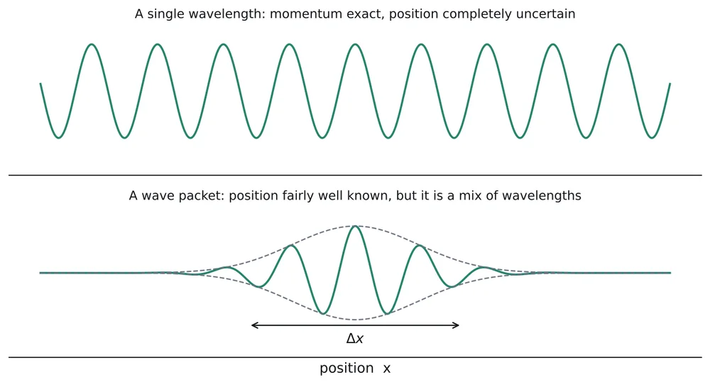
How a wave packet is formed. A wave packet is formed by the superposition (adding together) of a large number of waves of slightly different wavelengths and frequencies. In one small region the waves are in step and reinforce each other, which gives a large amplitude. Away from that region they go out of step and cancel, so the amplitude dies away.
- The larger the number of component waves (the wider the range of wavelengths), the smaller the length of the wave packet.
- The smaller the number of component waves, the longer the packet.
When the particle moves, the wave packet moves as a whole.
Phase velocity and group velocity
Two different velocities describe a wave packet:
- The phase velocity is the velocity of the individual component waves (the crests inside the packet).
- The group velocity is the velocity with which the wave packet as a whole (its envelope) moves.
The group velocity is equal to the velocity of the particle, so it is also called the particle velocity. It is the group, not the individual waves, that carries the particle along.
From wave packets to uncertainty
This picture leads directly to the uncertainty principle:
- If the wave function is a single sine wave of wavelength , the momentum is known exactly. But has the same value all over space, so the position at a given time cannot be determined. The particle is "spread out" in space: exact momentum means a very large uncertainty in position.
- If the wave function is a narrow packet of width , then is zero everywhere except in that region, so the position is known to within . But the packet is formed by the interference of a large number of waves of slightly different wavelengths. Since can take any value in that range, the momentum can also take a range of values. So there is an uncertainty in momentum .
- For a narrower packet the number of component waves must be larger, so is larger.
Key idea. You cannot make and both small at the same time. This trade-off is not a fault of our instruments. It is part of the wave nature of matter. It is Heisenberg's uncertainty principle (next page).
Watch out. The individual waves inside a packet (phase velocity) and the packet itself (group velocity) move at different speeds. When an exam asks for the speed of the particle, it is the group velocity.
Page 8 of 15
Heisenberg's uncertainty principle
Statement
When we treat a moving particle as a wave group, there are basic limits to the accuracy with which we can measure particle properties such as position and momentum.
Heisenberg's uncertainty principle. It is impossible to know both the position and the momentum of a particle exactly at the same time. If is the uncertainty in the position and the uncertainty in the corresponding component of momentum (), then
where , so that .
In simple words: the product of the uncertainty in position and the uncertainty in momentum can never be smaller than . The more precisely one is known, the less precisely the other can be known.
Other conjugate pairs
A pair of variables connected by an uncertainty relation is called a conjugate pair. Besides position and momentum, the important pairs are energy and time, and angular momentum and angular position:
Here and are the uncertainties in finding the energy and time, and and are the uncertainties in the angular momentum and the angle.
There is no uncertainty relation between and a component of momentum other than the component. For example, and can both be known exactly at the same time.
Note on the source. One lecture set wrote these relations with on the right (, , ) and the other with . The exact lower limit is , used in all these notes. Some textbooks write or even because they make an estimate of the order of magnitude. Then the answers change by a factor of 2 or . Write which form you use.
What the principle does and does not say
- It is not about poor instruments or experimental error. Even with perfect instruments, cannot be smaller than . It is a property of nature, coming from the wave nature of matter.
- It applies to simultaneous knowledge. You can measure position very precisely, but then the momentum becomes very uncertain, and the other way round.
- Because is tiny, the limits matter only on the atomic scale. For everyday objects the uncertainties are far too small to notice.
Why we never notice it in everyday life
Example 1. A bullet of mass moves with a speed of . The speed is measured to an accuracy of . How precisely can the position of the bullet be found?
The uncertainty in speed is of :
The uncertainty in momentum is
So
This uncertainty is far smaller than even the size of an atom (about ), so for a bullet it is completely negligible.
Note on the source. The lecture notes gave . When we calculate with , we get .
Example 2. An electron in an atom. An electron is confined within an atom of size about . Find the minimum uncertainty in its speed.
An uncertainty of more than half a million metres per second. For an electron in an atom, the uncertainty principle is very large, and the idea of a definite orbit with a definite speed breaks down.
Watch out. Change a percentage accuracy into an actual before multiplying by the mass, and use the mass in kilograms. Also remember that comes out as a minimum (), not an exact value.
Page 9 of 15
Applications of the uncertainty principle
Planck's constant is so small that the limitations given by the uncertainty principle are important only at the subatomic level. On that scale, the principle is a powerful tool for understanding many phenomena.
1. Electrons cannot exist inside the nucleus
In the early days, people thought that the electrons coming out of a nucleus as rays in radioactivity actually existed inside the nucleus before they were emitted. The uncertainty principle shows that this is impossible.
Step 1: the uncertainty in position. The diameter of a nucleus is typically about . If an electron existed inside it, the maximum uncertainty in its position would be the size of the nucleus:
Step 2: the minimum uncertainty in momentum.
Step 3: the minimum momentum. If this is the uncertainty in the momentum, the momentum itself must be at least as large:
Step 4: the minimum energy. At such a large momentum the electron moves at nearly the speed of light, so its rest-mass energy can be neglected and its kinetic energy is about :
Step 5: compare with experiment. An electron inside the nucleus would need a kinetic energy of at least about . But the electrons emitted in decay have energies of only a fraction of this, a few MeV at most. Hence electrons do not exist inside the nucleus. The electrons emitted in decay are created at the moment of decay, when a neutron changes into a proton.
Note on the source. One lecture set used with taken as the nuclear radius, and got and about . The other used and got . In both cases the conclusion is the same, because both values are far above the energies seen in decay.
2. Natural width of spectral lines (natural line broadening)
When excited atoms return to the ground state, they emit radiation. The emitted lines do not have a perfectly sharp frequency. Each line has a small spread of frequencies, called its natural width. The uncertainty principle explains this.
Step 1: the uncertainty in time. The average time between the excitation of an atom and the moment it radiates is called the lifetime of the excited state. It is typically about . This is the uncertainty in the time of the de-excitation:
Step 2: the uncertainty in energy. From ,
Step 3: the uncertainty in frequency. Since , :
So the emitted frequency is not sharp: the spectral line has a finite width of a few megahertz. The shorter the lifetime of the excited state, the broader the line.
Note on the source. The lecture set that used got for the same lifetime. It differs from only by the factor of 2 in the convention.
Key idea. Both applications use the same idea: a quantity confined to a small range ( or ) forces a large spread in its conjugate ( or ).
Watch out. Use (with ), not . If you combine it with , you get the neat result , which is worth remembering.
Page 10 of 15
The time-dependent Schrödinger equation
The idea
How can we find for a particle? The answer is the Schrödinger equation. It is to quantum mechanics what Newton's second law is to classical mechanics: given the forces acting (described by the potential energy ), it tells how the wave function behaves in space and time.
The Schrödinger equation cannot be derived from older physics. We get it by starting from the wave function of a free particle and using Planck's relation and de Broglie's relation . The equation we reach is then taken as the general law, valid for any potential. Two equivalent methods are given below. Learn one thoroughly. The second one is useful because it also gives the energy and momentum operators.
Derivation, route 1 (differentiating twice)
Consider a particle moving in the direction with momentum and energy . Its wave function is (see the free-particle page)
Step 1: differentiate (1) with respect to . Only the exponent depends on , and its derivative is :
Multiply both sides by . Since :
Step 2: differentiate (1) twice with respect to . Each differentiation brings down a factor :
Multiply both sides by :
Step 3: total energy. The total energy of the particle is the sum of its kinetic energy and potential energy . With :
Multiply by :
Step 4: put (2) and (3) in (4).
This is the time-dependent Schrödinger equation in one dimension. It is the most general form of the Schrödinger equation. and may depend on both position and time, which is why it is called time-dependent.
Derivation, route 2 (energy and momentum operators)
Start from the same wave function, .
Differentiating partially with respect to :
(using ). Differentiating partially with respect to :
Equations (6) and (7) say that, when they act on , energy and momentum can be replaced by operators:
Energy and momentum operators.
These are used to find the energy and momentum of a particle when its wave function is known.
Now write the total energy, , multiply by , and replace and by their operators ( means applying the momentum operator twice):
Since ,
which is equation (5) again.
Three dimensions
If depends on , and , the second derivative is replaced by the sum of all three:
where is the Laplacian operator.
What does
The potential energy function represents the effect of the surroundings on the particle. Any restriction on the motion of the particle (walls, barriers, the attraction of a nucleus) appears in . Once is known, the Schrödinger equation can be solved for the wave function of the particle, and from we get and all the other physical quantities.
Watch out. Be careful with the signs: there is a minus sign in front of , and (not ) on the left. They come from and from multiplying by . In an exam, write each step. Examiners give marks for the steps, not only for the final equation.
Page 11 of 15
The time-independent Schrödinger equation
The idea
In many situations, the potential energy of the particle does not depend on time. The forces acting on the particle, and hence , change only with the position of the particle, . The particle is then in a steady state. When this is true, the Schrödinger equation can be simplified by separating the wave function into a part that depends only on position and a part that depends only on time. The result is the steady-state or time-independent form.
Derivation
Step 1: separate the wave function. Start from the free-particle wave function and split the exponential into two factors:
Let , a function of position only (it is sometimes written or ). Then
So the wave function has a time-independent part and a time-dependent part .
Step 2: differentiate (1) with respect to . does not depend on , so only the exponential is differentiated:
Step 3: differentiate (1) twice with respect to . The exponential does not depend on , so only is differentiated:
Step 4: put in the time-dependent equation. The time-dependent Schrödinger equation is
Putting (1), (2) and (3) in (4):
On the left, , so
Step 5: cancel the time factor. Divide throughout by , which is never zero:
Step 6: rearrange. Take everything to one side:
and multiply through by :
This is the time-independent Schrödinger equation in one dimension. Since depends only on , there is no need for partial derivatives. Ordinary derivatives are used.
Three dimensions
Stationary states
For a steady state, the probability density is
because . So the probability density does not change with time. This is why these solutions are called stationary states. All the problems in this module (the box and the barrier) use the time-independent equation, because their potentials do not change with time.
Key idea. The time-independent equation can also be written as : some operator acting on gives a number times . Only certain values of (the energy eigenvalues) allow acceptable solutions (the eigenfunctions). The particle in a box shows this clearly.
Watch out. An equivalent and equally correct way to write the result is (multiply through by ). Do not mix the two forms in the middle of a derivation.
Page 12 of 15
Particle in a one-dimensional box: solving the equation
The set-up
Consider a particle of mass moving inside a box along the direction, bouncing back and forth between two walls a distance apart. The walls at and are infinitely high (potential barriers that cannot be crossed), so the particle can never get past them, however much energy it has. This is the one-dimensional infinite square well potential, also called a particle in a one-dimensional box. The potential energy varies as:
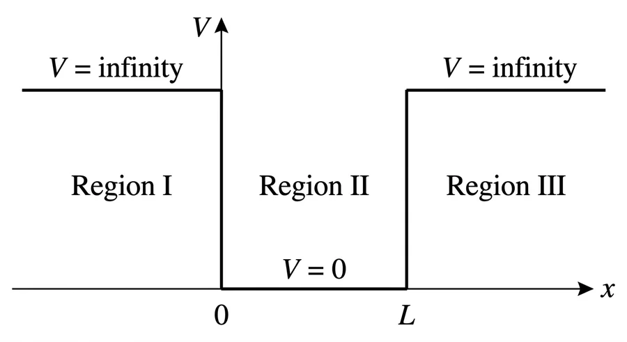
The position of the particle at any moment lies in . Since the particle cannot exist outside the box, the probability of finding it there is zero, so and hence for and . Our task is to find inside the box. Since the potential does not depend on time, we use the time-independent Schrödinger equation.
The equation inside the box
The time-independent Schrödinger equation is
Inside the box , so
Put
so the equation becomes
This is the equation of simple harmonic motion. Its general solution can be written in two equivalent ways.
Method A: sine and cosine form
The general solution of (2) is
with two constants and fixed by the boundary conditions. The wave function must be continuous, and it is zero outside the box, so it must vanish at both walls:
Boundary condition at :
So and
Boundary condition at :
We cannot have , because then everywhere and there would be no particle. So
Method B: exponential form
The general solution of (2) can also be written as
At : , so and
using .
At : . Since , , so again and . The wave function is
which is the same as Method A with the constant in place of . Both methods lead to
The wave function has several expressions, one for each value of . The th wave function is .
Why is not allowed
For , and everywhere inside the box. A wave function that is zero everywhere means the particle is not present at all, so is not allowed. Negative values of give the same functions with a minus sign (the same physical state), so we take
Watch out. The general solution has two constants. The boundary condition at removes the cosine (or makes ). The condition at quantises . Do not drop a constant at the start.
Note on the source. One lecture set wrote the general solution as "", where the second constant is missing. It is corrected above.
Page 13 of 15
Particle in a box: energy levels and wave functions
Allowed energy levels
The value of depends on the energy of the particle. From (1) and (4) on the previous page,
Since must be a whole number, the energy can take only certain values. Squaring both sides:
The second form uses , so . Each allowed energy is called an energy eigenvalue.
and in general : , , and so on. The number is called the quantum number.
Normalised wave functions
The wave function for level is . The square of the absolute value of the wave function gives the probability of finding the particle. Since the particle is certainly somewhere inside the box,
This is the normalisation condition. Putting :
Use :
Integrate each term:
So
The normalised wave function is
Each is an energy eigenfunction. For each value of there is an energy level and a corresponding wave function .
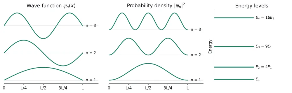
The figure shows the first three wave functions (left), the corresponding probability densities (middle) and the energy levels (right). As goes from to , the angle goes from to , so contains exactly half-wavelengths: one half-wave for , two for , three for .
What the solution tells us
- Energy is quantised. Inside the potential well, the particle can have only the discrete energies , not any arbitrary value. This is the origin of energy levels in atoms.
- Zero-point energy. The lowest energy is , not zero. This minimum is called the zero-point energy. A confined particle can never be completely at rest. (This agrees with the uncertainty principle: if the particle is confined to , there is a spread in momentum and hence some kinetic energy.)
- The levels are not equally spaced. , so the gaps increase: , , , …
- Preferred positions. In the ground state () the probability of finding the particle is greatest at the centre (). For the maxima are at and , a quarter and three quarters of the way across, and the probability at the centre is zero (a node). For the maxima are at , and . Classically every position would be equally likely.
- Smaller box, larger energies. and . For a large box or a heavy particle, the levels are so close together that the quantisation cannot be noticed, and the classical picture is recovered.
Key idea. When a particle is confined in a potential well, we get (i) certain preferred positions of maximum probability, (ii) only certain discrete energy levels, and (iii) a minimum energy that the particle must have.
Worked examples
Example 1. Find the ground-state energy of an electron in an infinitely deep box of width .
The next levels are and .
Example 2. In Example 1 the electron drops from to and emits a photon. Find the wavelength of the photon.
(using ). This is in the far ultraviolet.
Example 3. Find the ground-state energy of an electron in a box of width .
The box is 10 times wider than in Example 1, and , so the energy is 100 times smaller:
Example 4. An electron in a box of width is in its first excited state. Find the probability of finding it in the central half of the box.
The first excited state is . The central half runs from to :
The sine term is , so
For comparison, in the ground state () the same central half has probability , because the particle is concentrated near the centre.
Example 5. A particle is in the ground state of a box of width . Find the probability of finding it between and .
Only about 9 %, much less than the 25 % a classical particle would have, because the ground-state wave function is small near the walls.
Watch out. The quantum number starts at , so the "first excited state" is , not . Also, the energy depends on : if is doubled, the energy becomes four times.
Page 14 of 15
Quantum mechanical tunnelling
The idea
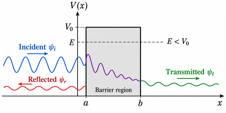
Consider a stream of particles, each of energy , falling on a potential barrier of height and width , with the energy less than the barrier height ():
- Classically, when a particle of lower kinetic energy approaches a higher potential barrier, it bounces back. It does not have enough energy to climb over, so it can never appear on the other side.
- Quantum mechanically, the wave function representing the particle does not vanish at the barrier. If we solve the time-independent Schrödinger equation in the three regions, the wave function is non-zero in all three regions I, II and III. So there is a finite probability that the particle goes through the barrier and is found beyond it.
Quantum mechanical tunnelling. The phenomenon of particles passing through potential barriers higher than their own energy is known as quantum mechanical tunnelling. It is purely a quantum effect, showing the wave property of quantum objects, and has no classical counterpart.
The wave function in each region
Region I (): incident and reflected waves. Here , so the solution is a travelling wave in each direction:
is the amplitude of the incident wave (moving right) and the amplitude of the reflected wave (moving left). The non-zero value of the wave function in region I is due to the incident particles and the particles reflected from the barrier.
Region II (): inside the barrier. Here , so is negative and the solution no longer oscillates. It decays exponentially with distance into the barrier, roughly as
The wave function is small at the far side of the barrier, but not zero. Since the probability of finding the particle is non-zero in region II, the particle can be inside the barrier, which is classically forbidden.
Region III (): the transmitted wave. Here again, so in general
where is the amplitude of the transmitted wave. But nothing comes back from the right, so there is no reflected wave in region III: and
Interpretation. A non-zero wave function in region III means there is a finite probability of finding particles there. The incident particles have less energy than the barrier height, so they could not have climbed over it. Also, the wave function is non-zero inside the barrier. So we conclude that the particles have reached region III by penetrating, or "tunnelling" through, the barrier.
Transmission coefficient
The probability of tunnelling is measured by the transmission coefficient . Since the probability of finding the particle is proportional to the square of the amplitude,
In classical physics when . In quantum mechanics it is a finite, non-zero quantity. For a barrier that is not too thin, it is approximately
so it falls off very rapidly:
- The wider the barrier ( larger), the smaller .
- The higher the barrier compared with the energy ( larger), the smaller .
- The heavier the particle ( larger), the smaller . So tunnelling is important for light particles such as electrons.
Example 1. An electron has energy less than the height of a barrier. Find the approximate transmission coefficient for a barrier of width (a) , (b) .
(a) , so .
(b) , so .
If the width is doubled, the tunnelling probability becomes about 170 times smaller. The scanning tunnelling microscope uses this extreme sensitivity to width.
Applications
- Tunnel diode (Module 4): electrons tunnel through a very thin depletion layer, giving a negative-resistance region used in high-frequency oscillators.
- Zener breakdown: in heavily doped p-n junctions, electrons tunnel through the thin depletion region at a sharp reverse voltage.
- Alpha decay: alpha particles inside a nucleus have less energy than the nuclear barrier, yet they escape by tunnelling.
- Scanning tunnelling microscope (STM): the tunnelling current between a sharp tip and a surface depends so strongly on the gap that it can map individual atoms.
- Josephson effect and SQUIDs: Cooper pairs tunnel through a thin insulating layer between two superconductors.
Watch out. Tunnelling does not mean the particle gains energy to go over the barrier. Its energy stays throughout. It appears on the far side with the same energy, only with a much smaller probability (amplitude). Also, is an approximation for a fairly wide barrier, not an exact result.
Page 15 of 15
Practice questions and formula sheet
Constants: , , , , .
Numerical problems
1. A certain excited state of a helium atom has an average lifetime of . What is the minimum uncertainty with which the frequency of the emitted radiation can be measured?
2. Calculate the uncertainty in the frequency of the emitted radiation if the uncertainty in time of an excited atom is .
3. The time gap between the excitation of an atom and the emission of radiation is . Find the uncertainty in the frequency of the radiation.
4. Find the energy of the ground state of an electron moving in an infinitely high potential box of width .
5. An electron confined in a one-dimensional box of width is known to be in its first excited state. Determine the probability of finding the electron in the central half.
, and integrating from to gives (worked on the energy-levels page).
6. Find the de Broglie wavelength of an electron accelerated through .
7. A bullet of mass moving at has its speed measured to . Find the minimum uncertainty in its position.
, , so .
8. Find the de Broglie wavelength of a neutron with kinetic energy ().
9. An electron is confined to a region of size . Find the minimum uncertainty in its speed.
, so .
10. For an electron in a box of width , find the wavelength of the photon emitted in the transition .
, so .
Note on the source. The lecture sheets used in one place and in another. With , as above. With every frequency width would be twice as large.
Questions asked in KTU exams
Short answer
- What is tunnel effect? What is quantum mechanical tunnelling?
- State and explain Heisenberg's uncertainty principle.
- What are the characteristics of a well-defined wave function?
- A well-behaved wave function is normalised. Why?
- Give the probability interpretation of the wave function.
- Explain the absence of electrons in the nucleus on the basis of the uncertainty principle.
- What is meant by a wave function? Write its normalisation condition.
- How do you account for natural line broadening on the basis of Heisenberg's uncertainty principle?
Essay
- Write the Schrödinger equation for a particle trapped in a one-dimensional box of width and solve it to obtain the energy eigenvalues and wave functions.
- State the uncertainty principle. Explain the absence of electrons inside the nucleus using this principle.
- Starting from the time-dependent equation, derive Schrödinger's time-independent wave equation.
- Formulate Schrödinger's time-dependent equation starting from a plane wave equation, using de Broglie's formula and Einstein's relation for photon energy.
Formula sheet
Matter waves and the wave function
| de Broglie wavelength | |
| Electron through volts | |
| Free-particle wave function | , with , |
| Probability density | |
| Probability in a region | |
| Normalisation |
Uncertainty principle
| Position and momentum | |
| Energy and time | |
| Angular momentum and angle | |
| Natural line width | |
| Electron in nucleus |
Schrödinger equation
| Time-dependent | |
| Time-independent | |
| Three dimensions | |
| Operators | , |
Particle in a box and tunnelling
| Energy levels | , |
| Wave functions | |
| Zero-point energy | |
| Level ratios | : |
| Transmission coefficient | , |