
Page 1 of 8
Module 4 overview
This module surveys the main algorithm design strategies. Each strategy is a general plan for building a solution; choosing the right one is often more important than the programming that follows.
| Strategy | Core idea | Typical example |
|---|---|---|
| Brute force | Try every candidate | Padlock combinations |
| Divide and conquer | Split, solve recursively, combine | Merge sort |
| Dynamic programming | Solve overlapping sub-problems once and reuse them | Fibonacci numbers |
| Greedy | Take the best-looking choice at each step | Activity selection |
| Randomized | Use random choices or simulation | Coupon collector, hat check |
All code is Python 3 and can be run as written; output comments show the expected result.
Key idea. Before choosing a strategy, ask how the problem decomposes, whether its sub-problems overlap, and whether an exact answer is required.
Page 2 of 8
Before choosing a strategy
A problem should be examined before any algorithm is chosen. Check that it is:
- Clearly defined. You can state the current situation, the goal, the possible ways to reach it, and the obstacles.
- Computable. The required calculations are feasible within a reasonable time and processing capacity.
- Understood in terms of data. You know what types of data are involved and how much storage they need.
- Suitable for decomposition and abstraction. These two techniques are the key to tackling complex problems: decomposition splits a problem into parts, and abstraction hides the details that do not matter for the current part.
Page 3 of 8
Brute-force approach
A brute-force (or exhaustive search) algorithm takes the most direct route: it generates every candidate and checks each one until the target is found. It makes no attempt to reduce the number of operations.
- Simple. Easy to design, easy to reason about, and usually correct by construction.
- Common in searching. The goal is to find an object among a list of candidates.
- Ignores problem structure. A smarter search would use the structure to discard many candidates early. Entering an unfamiliar grocery store, you would walk straight to the frozen-food aisle rather than inspect every aisle; brute force inspects them all.
- Costly for large problems. The search space is never reduced, so running time grows quickly with input size.
Example: padlock combination
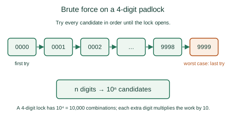
A padlock has a 4-digit code. Brute force tries 0000, 0001, 0002, and so on up to 9999. An -digit lock has combinations, so the 4-digit lock has .
def crack_lock(secret, digits=4):
    """Return the number of attempts needed to find the secret code."""
    for attempts, guess in enumerate(range(10 ** digits), start=1):
        if f"{guess:0{digits}d}" == secret:
            return attempts

print(crack_lock("0002"))  # 3
print(crack_lock("9999"))  # 10000  (worst case)
Watch out. Adding one digit multiplies the work by 10. Brute force is fine for small search spaces but quickly becomes impractical.
Page 4 of 8
Divide-and-conquer approach
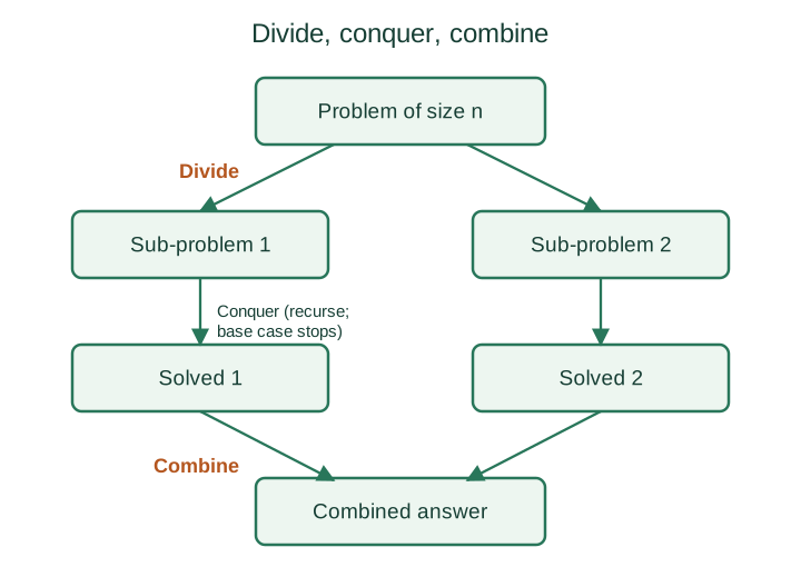
Divide and conquer solves a problem in three steps.
- Divide. Split the problem into smaller sub-problems of the same kind. Keep dividing until the pieces are small enough to solve directly.
- Conquer. Solve each sub-problem. This is normally done by recursion, which stops at a base case: a sub-problem so small that it is solved with basic operations and not divided further.
- Combine. Use the solutions of the sub-problems to build the solution of the original problem.
Recursion in divide and conquer
A recursive function calls itself on a smaller input. It keeps shrinking the problem until the base case is reached, and then the returned values are used to solve the larger problems on the way back.
Example: merge sort
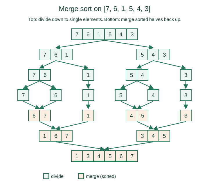
Merge sort follows the pattern exactly. To sort elements:
- Divide the sequence into two subsequences of about elements each.
- Conquer by sorting each subsequence recursively. A sequence of one element is already sorted (the base case).
- Combine by merging the two sorted subsequences into one sorted sequence.
def merge_sort(items):
    if len(items) <= 1:                  # base case
        return items
    middle = len(items) // 2
    left = merge_sort(items[:middle])    # divide + conquer
    right = merge_sort(items[middle:])
    return merge(left, right)            # combine

def merge(left, right):
    result, i, j = [], 0, 0
    while i < len(left) and j < len(right):
        if left[i] <= right[j]:
            result.append(left[i]); i += 1
        else:
            result.append(right[j]); j += 1
    return result + left[i:] + right[j:]   # one of these is empty

print(merge_sort([7, 6, 1, 5, 4, 3]))  # [1, 3, 4, 5, 6, 7]
Merge sort halves the list about times and does merging work at each level, so it runs in time.
Advantages
- Simplifies difficult problems by reducing them to smaller, manageable ones.
- Leads to efficient algorithms such as merge sort and quick sort.
- Uses memory caches well. Once the pieces are small they fit in cache, avoiding slower main-memory access.
- Can improve numerical accuracy in some computations that involve rounded arithmetic.
- Suits parallel execution. Independent sub-problems can run on different processor cores or machines.
Disadvantages
- Recursion overhead. Function calls cost time and memory, which can outweigh the benefit.
- More complex for large inputs. Many recursive calls can make a solution harder to follow than a plain loop.
- Overkill for simple tasks. Adding a list of numbers is simpler and faster with a loop.
Page 5 of 8
Dynamic programming approach
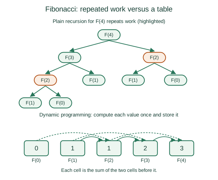
Dynamic programming (DP) is worthwhile when a problem has overlapping sub-problems: the same sub-problem is needed again and again. Instead of recomputing it, DP stores each result in a table (or array) and reuses it. This is called memoization when done top-down; retrieving a stored value takes constant time, .
DP is commonly applied to optimization problems, where many solutions are possible, each with a cost, and the goal is the solution of smallest cost (the optimal solution). For problems with overlapping sub-problems it avoids redundant work and still guarantees an optimal answer.
Example: Fibonacci series
Each Fibonacci number is the sum of the two before it: , , and for . The first five terms are 0, 1, 1, 2, 3.
Plain recursion recomputes values such as many times. DP computes each value once and reads earlier results from the table.
def fib_table(n):
    """Bottom-up dynamic programming."""
    if n < 2:
        return n
    table = [0, 1]
    for i in range(2, n + 1):
        table.append(table[i - 1] + table[i - 2])
    return table[n]

def fib_memo(n, memo=None):
    """Top-down: recursion plus memoization."""
    memo = {} if memo is None else memo
    if n < 2:
        return n
    if n not in memo:
        memo[n] = fib_memo(n - 1, memo) + fib_memo(n - 2, memo)
    return memo[n]

print([fib_table(i) for i in range(5)])  # [0, 1, 1, 2, 3]
print(fib_memo(50))                      # 12586269025
Recursion versus dynamic programming
DP is mostly applied to recursive algorithms, but not every recursive algorithm can use it. DP helps only when sub-problems overlap, as in Fibonacci. Merge sort's sub-problems (different halves of the list) never overlap, so it stays a pure divide-and-conquer algorithm.
Key idea. Divide and conquer: sub-problems are independent. Dynamic programming: sub-problems overlap, so store their answers.
Page 6 of 8
Greedy approach
A greedy algorithm builds a solution step by step, always choosing the option with the best immediate (local) value, and never reconsidering. It uses only a small part of the problem's information at each step.
- Simple and fast. Each local decision needs very little computation.
- Not always optimal. A choice that looks best now can be costly later, so a greedy strategy does not guarantee the best overall solution for general problems.
- Optimal for some problems. When local decisions line up with the global optimum, greedy gives the best answer. Activity selection is the standard example.
Characteristics
- There is an ordered list of resources, each with a cost or value, which expresses the constraints of the system.
- At each step, take as much of the resource as the constraint allows.
- For example, in activity scheduling the costs are durations in hours, and the activities must be performed one after another.
Why use greedy?
- It reaches a feasible solution immediately, with no backtracking.
- It reduces the problem in a single pass, without combining many sub-solutions. In activity selection one scan over the activities is enough.
Example: activity selection
Select the largest set of activities that do not overlap. The greedy rule is to sort by finish time and always take the next activity that starts after the last chosen one finishes.
activities = [(1, 4), (3, 5), (0, 6), (5, 7), (8, 9), (5, 9)]   # (start, finish)

def select_activities(activities):
    chosen, last_finish = [], 0
    for start, finish in sorted(activities, key=lambda a: a[1]):
        if start >= last_finish:
            chosen.append((start, finish))
            last_finish = finish
    return chosen

print(select_activities(activities))  # [(1, 4), (5, 7), (8, 9)]
When greedy fails
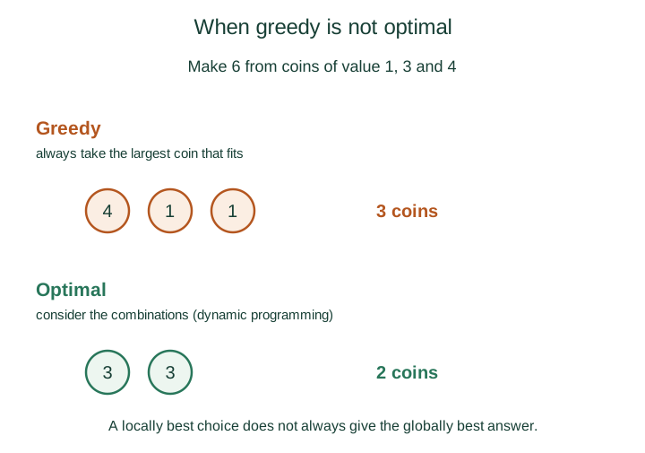
With coins of value 1, 3 and 4, making 6 greedily takes 4 then 1 then 1: three coins. The optimum is 3 + 3: two coins. The first choice looked best but ruined the rest.
Greedy versus dynamic programming
| Greedy | Dynamic programming | |
|---|---|---|
| Decision | Best local choice, made once | Solves sub-problems, then chooses among their results |
| Looks back? | No | Yes, uses stored sub-solutions |
| Optimal? | Only for some problems | Yes, when sub-problems overlap and combine correctly |
| Cost | Usually fastest | Needs a table of results |
Page 7 of 8
Randomized approach
A randomized algorithm uses random numbers to make some of its decisions. It is effective when there are many alternatives and most of them are "good", so finding the single best one is not worth the effort.
- Different runs on the same input can follow different paths and give different outcomes.
- Because no particular input is consistently bad, it reduces the chance of repeated worst-case behavior.
- Limitation: it does not improve the worst-case running time.
Applications
- Game-theoretic situations, to keep outcomes fair and unpredictable.
- Computer and information security, where unpredictability is needed.
- Computer games, to introduce variability.
Motivation
- Simplicity. Approximating by simulation can be easier than an exact deterministic solution.
- Large problem spaces. Randomness explores permutations and combinations without enumerating all of them.
- Fairness. Auctions and competitive settings avoid predictable results.
- Robustness. The method is not biased toward any particular kind of input.
- Mathematical guarantees. Probability theory (for example, expected values) shows that estimates become accurate in the long run, even though a single run is unpredictable.
Example 1: coupon collector
A company puts one of different coupons in each pair of jeans, chosen at random. Collecting all gives a free pair. On average, how many pairs must you buy?
import random

def simulate_coupon_collector(n, trials):
    total_jeans = 0
    for _ in range(trials):
        collected = set()
        jeans_bought = 0
        while len(collected) < n:
            collected.add(random.randint(1, n))   # buy jeans, get a random coupon
            jeans_bought += 1
        total_jeans += jeans_bought
    return total_jeans / trials

print(simulate_coupon_collector(10, 10000))  # about 29.3 (varies from run to run)
- Initialize
nand an empty set of collected coupons. - Simulate buying jeans until the set holds all
ncoupons, counting purchases. - Repeat for many trials and average the counts.
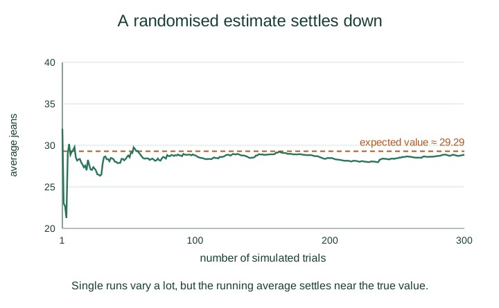
The exact expected value is , which is about 29.29 for . More trials bring the estimate closer to it.
Example 2: hat check
people leave their hats with a hat-check person. At the end of the party a different attendant returns the hats at random. What is the expected number of people who get their own hat back?
import random

def simulate_hat_problem(n, trials):
    total_matches = 0
    for _ in range(trials):
        hats = list(range(1, n + 1))   # hat i belongs to person i
        random.shuffle(hats)           # return hats at random
        total_matches += sum(1 for i in range(n) if hats[i] == i + 1)
    return total_matches / trials

print(simulate_hat_problem(10, 10000))  # about 1.0 (varies from run to run)
- Initialize
nand a random permutation of the hats for each trial. - Count how many people receive their own hat.
- Average over many trials.
The expected number of matches is exactly 1, whatever the value of .
Page 8 of 8
Comparing the strategies
| Strategy | Best when | Watch out for |
|---|---|---|
| Brute force | The search space is small, or correctness matters more than speed | Running time explodes as the input grows |
| Divide and conquer | Sub-problems are independent and easy to combine | Recursion overhead |
| Dynamic programming | Sub-problems overlap and an optimal answer is needed | Memory for the table |
| Greedy | A local choice is provably part of a global optimum | May be suboptimal; always verify |
| Randomized | Many "good" answers, or fairness and unpredictability matter | Results vary between runs; worst case unchanged |
Check your understanding
- Why does brute force become impractical as the number of digits grows?
- Which three steps make up divide and conquer, and what is a base case?
- Why can Fibonacci use dynamic programming but merge sort cannot?
- Give a case where a greedy choice is not optimal.
- Why does the average of a randomized simulation become more reliable with more trials?
References
- Algorithmic Thinking with Python, Ajeesh Ramanujan and Narasimhan T — source study material.
- Python tutorial: recursion and functions.
- Python library: random.