
Spectroscopy, radiation and molecular energy
This module moves from fundamental light–matter interactions to spectroscopy and instrumental analysis:
- Spectroscopy, radiation and molecular energy
- Transmittance, absorbance and the Beer–Lambert law
- Worked problems on absorbance and concentration
- UV–visible spectroscopy and electronic transitions
- Conjugation and predicting molecular transitions
- UV–visible spectrophotometer: instrument and applications
- Infrared absorption and types of vibration
- Counting vibrations: carbon dioxide, water and HCN
- Bond vibrations and force-constant calculations
- Reading IR spectra and studying hydrogen bonding
- Dielectric thermal analysis: principle, instrument and uses
- Scanning electron microscopy: signals, instrument and uses
- Revision sheet and practice problems
Interaction of radiation with matter
Spectroscopy
Spectroscopy is the study of how electromagnetic radiation interacts with atoms, ions, and molecules. Many spectroscopic methods provide rapid quantitative and qualitative analysis using minute sample quantities. Whether the sample can be recovered intact depends on the required sample preparation, incident radiation energy, and specific technique employed.
Electromagnetic radiation
Electromagnetic radiation consists of mutually perpendicular oscillating electric and magnetic fields propagating through space, characterised by wavelength (), frequency (), or wavenumber (). The energy of a single photon is directly proportional to frequency and inversely proportional to wavelength:
where:
- is Planck's constant ()
- is the speed of light in vacuum ()
- is frequency in hertz ( or )
- is wavelength (commonly in or )
- is wavenumber (commonly in )
Across the electromagnetic spectrum—from radio waves through microwaves, infrared (IR), visible light, ultraviolet (UV), X-rays, to gamma rays—wavelength decreases progressively while frequency and photon energy increase. When calculating energies, ensure compatible length units: when using in , convert to metres () and to ().
Fundamental radiation–matter processes
When electromagnetic radiation encounters matter, three primary interactions can occur:
- Absorption: An atom or molecule absorbs a resonant photon and transitions from a lower energy state () to an allowed higher energy state (), where . Typical absorption methods include UV–visible, infrared, microwave, and nuclear magnetic resonance (NMR) spectroscopy.
- Emission: An excited species relaxes from a higher energy state () to a lower energy state () by releasing a photon of matching energy . Key examples include atomic emission and fluorescence spectroscopy.
- Scattering: Incident radiation is redirected into new directions upon colliding with matter without necessarily undergoing direct resonant absorption. In Raman spectroscopy, inelastic light scattering occurs, causing scattered photons to gain or lose discrete amounts of vibrational or rotational energy.
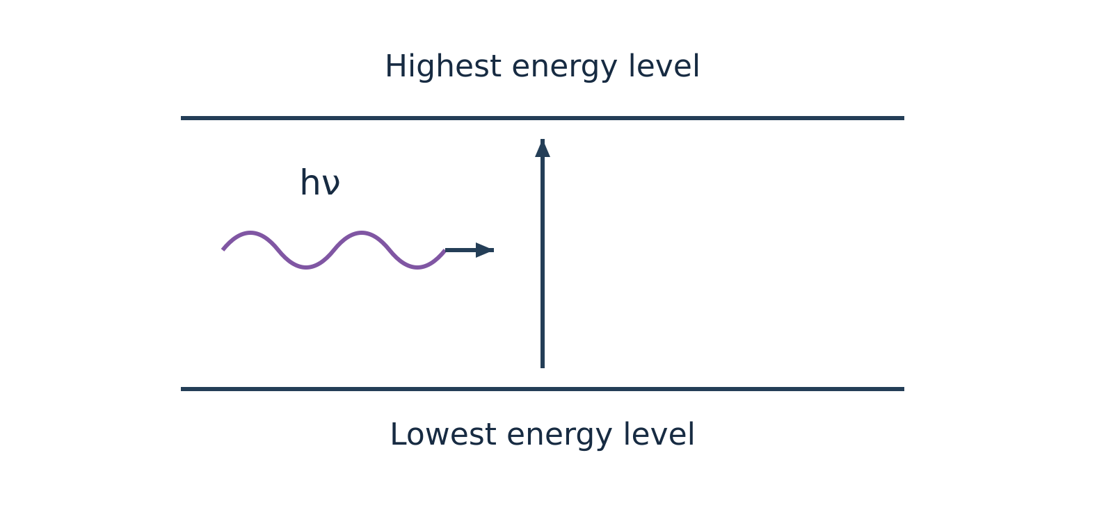
Figure 1a: Qualitative schematic of photon absorption driving an upward transition from a lower to a higher energy state.
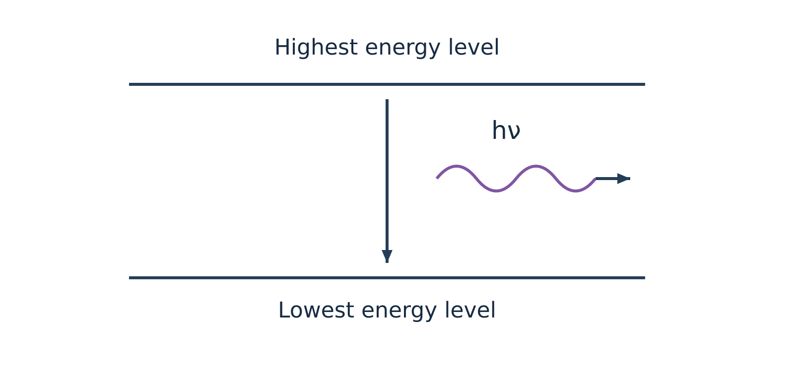
Figure 1b: Qualitative schematic of photon emission during relaxation from a higher to a lower energy state.
Watch out. Quantum mechanical transitions take place between any permitted lower and higher energy states that satisfy the specific selection rules—not exclusively between the absolute ground and highest excited levels. Furthermore, Raman spectroscopy is an inelastic scattering process, not an emission technique; and atomic force microscopy (AFM) is a mechanical scanning probe method, not optical spectroscopy.
Molecular energy levels and the Born–Oppenheimer approximation
A molecule distributes its total energy among translational, rotational, vibrational, and electronic degrees of freedom:
Translational energy
Translational energy () arises from the unconstrained displacement of the molecule's centre of mass through three-dimensional space. Because translational quantum states in macroscopic containers are spaced by infinitesimal energy increments, they form an effective continuum and are separated from quantised internal states.
Born–Oppenheimer approximation
The Born–Oppenheimer approximation states that because heavy atomic nuclei move much more slowly than light electrons, electronic motion can be treated independently of nuclear motions. Under this approximation, the total internal molecular energy () separates into distinct electronic, vibrational, and rotational contributions:
| Energy Level Type | Physical Origin | Typical Spectral Region | Typical Units Used | Key Requirement |
|---|---|---|---|---|
| Electronic () | Promotion of bonding or non-bonding valence electrons between molecular orbitals | Ultraviolet–visible (UV–vis) | Wavelength in () | Chromophore / accessible empty orbitals |
| Vibrational () | Periodic stretching and bending of chemical bonds with fixed centre of mass | Infrared (IR) | Wavenumber in () | Dynamic change in molecular dipole moment () |
| Rotational () | End-over-end rotation of the molecule about an axis passing through its centre of mass | Microwave | Frequency () or wavenumber () | Permanent electric dipole moment () |
The energy separations between adjacent quantum states follow a strict hierarchical order:
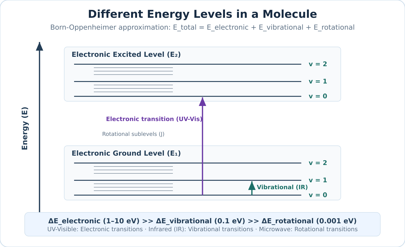
Figure 2: Qualitative diagram of nested molecular energy levels. Each electronic state contains multiple vibrational levels (), and each vibrational level contains closely spaced rotational levels (). Spacing is schematic and not drawn to scale.
Atomic versus molecular spectra
The presence of chemical bonds fundamentally alters the nature of spectral transitions:
Atomic spectra
Atomic spectra arise from isolated gaseous atoms that possess only electronic degrees of freedom and lack chemical bonds, meaning they have no vibrational or rotational sublevels. Electronic transitions between discrete atomic orbitals therefore yield narrow, sharp line spectra (subject to Doppler and natural lifetime broadening).
Molecular spectra
Molecular spectra arise because molecules possess vibrational and rotational sublevels nested within each electronic state. An electronic transition in a molecule is accompanied by simultaneous vibrational and rotational co-transitions (vibronic and rovibronic coupling). In condensed phases or solution, rapid intermolecular collisions and solvent-solute interactions further broaden these closely packed transitions into broad band spectra.
Self-check questions
-
Question: Why does a gaseous atom produce sharp spectral lines whereas a molecule in solution produces broad UV–visible absorption bands?
Answer: Gaseous atoms undergo electronic transitions purely between unperturbed, discrete atomic energy levels, yielding sharp lines. Molecules have vibrational and rotational energy sublevels nested within each electronic state. Simultaneous transitions across these closely spaced sublevels, combined with collisional dephasing and solvent interactions in solution, smear individual transitions into continuous, broad absorption bands. -
Question: Arrange microwave, ultraviolet, and infrared radiation in order of increasing photon energy and state the primary molecular transition promoted by each.
Answer: In order of increasing energy:- Microwave: Promotes rotational transitions.
- Infrared: Promotes vibrational stretching and bending transitions.
- Ultraviolet: Promotes electronic transitions between valence molecular orbitals.
Transmittance, absorbance and the Beer–Lambert law
When a beam of electromagnetic radiation passes through a sample solution, molecules absorb photons whose energies match allowed internal transitions. Consequently, the intensity of the emerging beam is lower than that of the entering beam. Quantitative absorption spectroscopy measures this attenuation to determine how much absorbing substance is present.
Transmittance and Absorbance
Consider a parallel beam of monochromatic radiation with incident intensity passing through a sample cell (cuvette) of path length containing an absorbing solution of molar concentration . The radiation emerges with transmitted intensity .
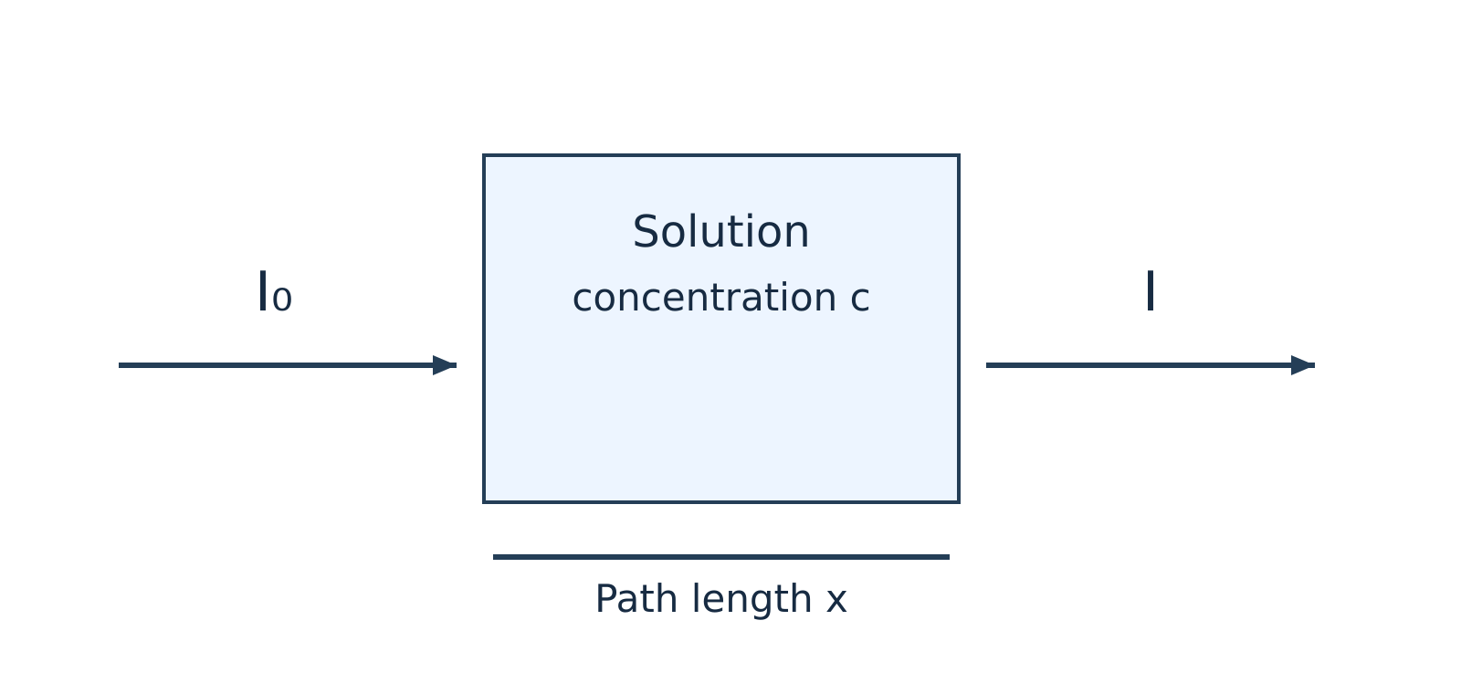
Figure 1: Attenuation of an incident light beam () passing through an absorbing solution of concentration and path length (or ).
Transmittance
Transmittance () is the fraction of incident radiation that successfully passes through the sample:
Because is a ratio of two intensities, it is dimensionless and ranges from (complete absorption) to (no absorption). Instrument readouts often express this value as percentage transmittance ():
Transmittance decreases exponentially as concentration or path length increases.
Absorbance
Absorbance (), historically termed optical density, is defined as the base-10 logarithm of the reciprocal of transmittance:
To convert directly from percentage transmittance to absorbance, substitute :
Like transmittance, absorbance is a dimensionless quantity.
Beer–Lambert Law and Derivation
Beer–Lambert Law
Beer–Lambert law states that when a parallel beam of monochromatic radiation passes through a homogeneous, non-scattering, dilute solution, the rate of decrease in radiation intensity () with respect to an infinitesimal thickness of the medium () is directly proportional to both the local intensity and the molar concentration of the absorbing species. It unifies Lambert's observation (attenuation scales with path length) with Beer's observation (attenuation scales with concentration).
Watch out. Many introductory notes state that the Beer–Lambert law applies only to "coloured" solutions. In reality, the law applies to any absorbing species—including colourless solutions that absorb strongly in the ultraviolet (UV) or infrared (IR) regions.
Derivation Steps
-
Set up the differential rate equation: Express the rate of intensity loss across an infinitesimal layer of thickness :
where is a proportionality constant dependent on the wavelength and the absorbing species.
-
Separate variables: Rearrange the equation to isolate intensity terms on the left and path length terms on the right:
-
Integrate across the cell boundaries: Integrate from the entrance boundary (, where intensity is ) to the exit boundary (, where intensity is ):
-
Evaluate the definite integrals:
-
Convert to common logarithms: Convert from natural logarithms () to decadic logarithms () using :
-
Define molar absorptivity: Define the molar absorption coefficient as . Substituting yields the standard integrated law:
(Note: Some texts and diagrams denote the cuvette path length using rather than , expressing the relationship as .)
Units of the Molar Absorption Coefficient ()
Molar Absorptivity
Molar absorption coefficient () (or molar absorptivity) is a fundamental optical property measuring how strongly a chemical species attenuates light at a specified wavelength, solvent, and temperature. Because absorbance is dimensionless, the dimensions of must cancel those of concentration and path length ().
| Convention | Concentration () | Path Length ( or ) | Unit of | Numerical Relationship |
|---|---|---|---|---|
| Standard Spectroscopy | (or ) | |||
| Decimetre Convention | () |
Watch out. Because , expressing path length in decimetres () simplifies the dimensional algebra (), which is why exam problems often use it. However, dividing by instead of makes the numerical value of in exactly times larger than the standard value in . Always state your chosen path-length unit explicitly.
Calibration and Analysis
For a fixed cuvette path length , plotting absorbance against molar concentration across a series of known standard solutions yields a linear relationship described by .
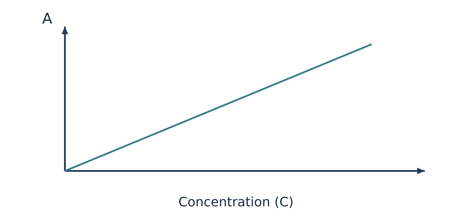
Figure 2: Ideal Beer–Lambert calibration plot of absorbance () versus concentration (), with slope equal to (or ).
Ideally, the calibration line passes through the origin with a slope of . Once established, the concentration of an unknown sample can be interpolated directly from the graph or calculated from a reference standard using the proportional ratio:
Spectroscopic Blank
Spectroscopic blank refers to an identical cuvette filled with pure solvent and all background reagents excluding the analyte. Because cuvette walls and solvent molecules reflect and absorb a small fraction of incident radiation, the spectrophotometer must be zeroed using a blank before sample measurement. This baseline correction minimizes solvent and cell contributions. If minor instrumental drift or reagent background persists, calibration data is fitted to a linear regression with an intercept ().
Assumptions and Deviations from Linearity
The linear relationship holds strictly only when specific physical, chemical, and instrumental constraints are satisfied:
- Monochromatic radiation: The incident radiation must consist of a narrow wavelength band over which is effectively constant. Broad polychromatic light or instrumental stray light causes severe negative deviations at high absorbance values.
- Dilute solutions: At high solute concentrations, inter-ionic and intermolecular electrostatic interactions perturb the electron charge distributions of the absorbing chromophore, altering . High concentrations also alter the solution's refractive index.
- Homogeneous, non-scattering medium: The solution must be clear and free from turbidity. Suspended colloidal particles scatter light away from the photodetector, generating artificially elevated apparent absorbance readings.
- Chemical stability: The absorbing species must not undergo concentration-dependent chemical equilibria (such as acid–base dissociation, association, tautomerism, or complexation) that alter the relative proportion of absorbing molecules upon dilution.
Self-Check Questions
-
Question: A solution transmits of incident monochromatic light at . What is its absorbance?
Answer: Using the conversion formula : -
Question: Why does a spectrophotometric calibration curve often bend downwards (negative deviation) at high analyte concentrations?
Answer: At elevated concentrations, solute–solute electrostatic interactions alter the molar absorptivity (), chemical equilibria may shift the active chromophore population, and instrumental stray light places an upper ceiling on accurately measurable absorbance.
Worked problems on absorbance and concentration
Strategy for Beer–Lambert Law Calculations
Quantitative spectrophotometry relies on the linear relationship between absorbance () and molar concentration () for dilute, homogeneous solutions measured with monochromatic light:
Here, is the molar absorption coefficient and is the optical path length of the sample cell (cuvette). When solving numerical problems, keep three physical principles in mind:
-
Higher absorbance means higher concentration, but lower transmittance. A more concentrated solution absorbs more photons, so less transmitted light () reaches the detector relative to the incident beam (). Therefore, as concentration increases, absorbance () increases while fractional transmittance () decreases.
-
Never confuse transmitted intensity with transmittance. Intensity () is radiative power per unit area, whereas fractional transmittance () is a dimensionless ratio between and , often expressed as percentage transmittance (). Because absorbance is logarithmic:
- Ratio methods eliminate constants under identical conditions. When a standard solution of known concentration () and an unknown sample () of the same chemical species are measured at the same wavelength, temperature, and solvent environment inside identical cuvettes (same and ), the constants cancel out:
| Quantity | Symbol | Common Laboratory Unit | Decimetre-Consistent Unit |
|---|---|---|---|
| Absorbance | Dimensionless | Dimensionless | |
| Fractional transmittance | Dimensionless () | Dimensionless () | |
| Concentration | () or | ||
| Path length | () | ||
| Molar absorption coefficient |
Watch out. Do not mix centimetres and decimetres when calculating . Because , keeping in gives in . Converting into () changes the numerical value of by a factor of and gives units of (since , never ).
Step-by-Step Worked Examples
Example 1: Calculating Absorbance and Molar Absorption Coefficient from Percentage Transmittance
Problem:
The percentage transmittance of a dye solution in ethanol is in a cell for monochromatic light of wavelength . Calculate the absorbance and the molar absorption coefficient in both and .
Solution:
-
Identify the given data and convert units:
- Concentration:
- Path length:
- Wavelength: (fixes the value of for this transition, though does not enter the arithmetic directly)
- Percentage transmittance: , so fractional transmittance (meaning for arbitrary intensity units, units pass through)
-
Calculate the absorbance ():
- Calculate the molar absorption coefficient () in standard laboratory units ():
Using and :
- Express in decimetre-consistent units ():
Using and :
Answer:
The absorbance is (dimensionless), and the molar absorption coefficient is (or ).
Example 2: Finding an Unknown Concentration by Direct Absorbance Ratio
Problem:
A standard dye solution of concentration shows an absorbance of at , while a test solution of the same dye shows an absorbance of under identical conditions (same cuvette and temperature). Find the concentration of the test solution.
Solution:
-
State the given quantities:
- Standard concentration:
- Standard absorbance:
- Test absorbance:
- Measurement wavelength:
-
Apply the Beer–Lambert law to both solutions:
Because the same dye is measured at the same wavelength () in the same cuvette, both and are identical for the two measurements:
- Solve for the unknown concentration ():
Notice that the test solution has a lower absorbance than the standard (), confirming physically that it must be more dilute ().
Answer:
The concentration of the test dye solution is .
Example 3: Colorimetric Determination of from Fractional Transmittance
Problem:
A standard solution of , after developing a red complex with excess ammonium thiocyanate (), shows a fractional transmittance of at . An unknown solution treated identically shows a fractional transmittance of at the same wavelength in the same cell. Calculate the concentration of the unknown solution. (Note: One course note transcription states while another states ; the arithmetic is independent of the numerical wavelength provided both standard and sample are measured at the exact same chosen wavelength.)
Solution:
-
Understand the chemical and optical conditions:
A colour-developing reagent () is added in excess under controlled conditions to form strongly absorbing red iron(III)–thiocyanate complexes. Calibration relates their response to the analytical iron concentration. Merely adding the same volume of reagent is not enough by itself; the reagent must be in sufficient excess, with identical matrix conditions and proper blank calibration, so that the complex speciation and effective remain constant across both solutions. -
List the given values:
- Standard concentration:
- Standard fractional transmittance:
- Unknown fractional transmittance:
-
Relate concentration to fractional transmittance:
Since and is constant across both measurements:
- Substitute the values and compute :
Watch out. Never take a direct linear ratio of transmittances (). Concentration is proportional to absorbance (), not to . Furthermore, because the unknown transmits more light (), it absorbs less light and must be less concentrated than the standard ().
Answer:
The concentration of the unknown solution is . Mass-concentration ratios are valid here because the standard and unknown use the same concentration basis; calculating a molar absorption coefficient requires molar concentration.
Self-Check Questions
-
Question: Solution X has and Solution Y of the same solute in the same cuvette has . Which solution is more concentrated, and by what factor?
Answer: Solution X is more concentrated because it transmits less light ( vs ). It is times as concentrated as Solution Y. -
Question: Why is the molar absorption coefficient numerically equal to ?
Answer: Because and , substituting these into the unit expression gives .
UV–visible spectroscopy and electronic transitions
UV–visible (UV–vis) spectroscopy
UV–visible (UV–vis) spectroscopy is an absorption spectroscopy technique that measures how molecules interact with electromagnetic radiation in the ultraviolet () and visible () regions. Because photons in these spectral bands carry sufficient energy to promote valence electrons from lower-energy ground-state molecular orbitals to higher-energy excited-state molecular orbitals, an absorption spectrum recorded in this region is known as an electronic spectrum. It is conventionally represented as a plot of absorbance () or molar absorptivity () as a function of wavelength (, expressed in ).
For practical chemical analysis, the ultraviolet–visible range is divided into three distinct operational domains:
- Far (vacuum) UV region (): High-energy radiation where atmospheric oxygen and common optical materials absorb strongly. Standard measurements require specialized vacuum chambers, nitrogen purge systems, and high-purity fluoride optics.
- Near-UV region (): Accessible using standard quartz (fused silica) cuvettes and standard benchtop optical paths in ambient air.
- Visible region (): Directly perceived by the human visual system. A substance appears coloured when it selectively absorbs specific visible wavelengths and transmits or reflects the complementary wavelengths.
The standard introductory benchtop working window spans , though modern research spectrophotometers often extend beyond these boundaries.
Molecular orbitals and electronic transitions
When a molecule absorbs an incident photon matching the transition energy , an electron is promoted from an occupied molecular orbital to an unoccupied antibonding orbital according to the Planck–Einstein relation:
where:
- is Planck's constant ()
- is the speed of light in a vacuum ()
- is the absorbed photon wavelength ()
Ground-state valence electrons reside in three principal classes of molecular orbitals:
- Sigma () bonding orbitals: Low-energy, symmetrical orbitals housing strongly localized electrons that constitute single covalent bonds.
- Pi () bonding orbitals: Higher-energy bonding orbitals formed by the lateral overlap of atomic orbitals, housing mobile electrons in double and triple bonds.
- Non-bonding () orbitals: Orbitals containing localized, unshared valence lone pairs on heteroatoms such as oxygen (), nitrogen (), sulfur (), and the halogens ().
The higher-energy unoccupied levels are antibonding orbitals, designated as (pi-star) and (sigma-star). In simple organic frameworks, orbital energy typically ascends in the order . This hierarchy establishes four fundamental electronic promotions:
(Note: While this relative ordering provides a reliable heuristic, exact orbital energies depend on atomic electronegativity and molecular geometry.)
The four principal transition types
- transitions: Promotion of an electron from a bonding orbital into an antibonding orbital. Due to the high thermodynamic stability and bond strength of single covalent bonds, this process requires high energy, producing absorption bands deep in the far-UV region (). Fully saturated hydrocarbons (such as methane, ethane, and cyclohexane) exhibit exclusively transitions and are completely transparent across the routine analytical window.
- transitions: Promotion of a non-bonding lone-pair electron () into an unoccupied orbital. Saturated molecules bearing heteroatoms with lone pairs (e.g., alcohols, ethers, amines, alkyl halides) undergo these transitions. They require less energy than transitions and generally occur between and . Highly electronegative systems (methanol, methylamine) absorb in the far UV below , whereas heavier, polarizable systems (such as iodoalkanes) extend well into the accessible near-UV region above .
- transitions: Promotion of an electron from a bonding orbital into an antibonding orbital in unsaturated compounds (alkenes, alkynes, aromatics, carbonyls). Isolated carbon–carbon double bonds absorb in the far UV (ethene exhibits ), whereas conjugated polyene systems shift into the routine region. Most transitions are symmetry- and spin-allowed, generating intense absorption bands (). However, symmetry-forbidden bands also exist, such as the weak benzenoid band centered at .
- transitions: Promotion of a heteroatom lone-pair electron into an unoccupied antibonding orbital in unsaturated systems containing heteroatoms (aldehydes, ketones, carboxylic acids, esters, nitro groups). In simple carbonyl compounds, the and orbitals are mutually perpendicular, making the electric-dipole transition formally symmetry-forbidden. Molecular vibrations slightly disrupt molecular symmetry (vibronic coupling), permitting weak absorption () at longer wavelengths () relative to bands.
| Transition | Structural Requirement | Representative Examples | Typical Spectral Region | Relative Absorption Intensity |
|---|---|---|---|---|
| Saturated single covalent bonds () | , , cyclohexane | Far UV () | Strong (outside routine benchtop window) | |
| Single bonds + heteroatom lone pairs | , , | Far UV to near UV () | Moderate to weak | |
| Multiple covalent bonds ( systems) | Ethene, 1,3-butadiene, benzene | Far UV (isolated) to (conjugated) | Usually strong (); occasionally weak | |
| Multiple bonds with heteroatom lone pairs | Acetone, ethanal, nitromethane | Near UV / visible () | Weak (; symmetry-forbidden) |
Watch out. Describing and transitions as "UV–vis inactive" is inaccurate. They do absorb UV radiation; however, their absorption maxima fall below , placing them outside the detection window of routine benchtop instruments operating in air.
Chromophores, auxochromes, and spectral shifts
Chromophore
An isolated functional group or structural unit within a molecule responsible for absorbing electromagnetic radiation in a defined spectral region. Although historically defined as an impartor of visible color, in modern spectroscopy a chromophore refers to any light-absorbing group, even if absorption occurs strictly in the ultraviolet region (e.g., , , , , benzene rings, and even -bond frameworks in the vacuum UV).
Auxochrome
A saturated functional substituent bearing non-bonding electron pairs (such as , , , , or halogens) that does not absorb significantly above on its own, but systematically alters both the wavelength and molar absorptivity when directly attached to a chromophore. Auxochromes delocalize their lone pairs into the adjacent system via resonance ( conjugation) or inductive effects, generally shifting absorption toward longer wavelengths and increasing band intensity.
Wavelength of maximum absorbance ()
The specific wavelength corresponding to the absorption peak of an electronic transition band. It serves as a diagnostic physical parameter governed by molecular conjugation, auxochromic substitution, and solvent interactions.
Spectral shifts and intensity modifications
Structural substitution or solvent changes produce four distinct spectral modifications:
- Bathochromic shift (Red shift): Displacement of an absorption band to a longer wavelength (lower excitation energy, smaller ).
- Hypsochromic shift (Blue shift): Displacement of an absorption band to a shorter wavelength (higher excitation energy, larger ).
- Hyperchromic effect: An increase in the molar absorptivity (), reflecting enhanced transition probability.
- Hypochromic effect: A decrease in the molar absorptivity (), reflecting suppressed transition probability.
Self-check questions
-
Which electronic transitions occur in propanone (acetone, ), and which transition occurs at the longest wavelength?
Answer: Propanone contains single and bonds, a double bond (), and non-bonding lone pairs () on the carbonyl oxygen atom. Consequently, it exhibits four possible promotions: , , , and . Because the transition possesses the smallest energy difference (), it absorbs photons of the lowest energy and therefore appears at the longest wavelength (). -
Why is the absorption band of an aldehyde significantly weaker than its absorption band?
Answer: The non-bonding orbital () of the carbonyl oxygen lies in the molecular plane, whereas the orbital is oriented perpendicular to the molecular plane. Because spatial orbital overlap between and is nearly zero, the electric-dipole transition integral is formally forbidden by symmetry selection rules. Weak absorption occurs only via vibronic coupling (molecular vibrations temporarily breaking local symmetry), yielding a low transition probability and a correspondingly low molar absorptivity (), compared to the fully symmetry-allowed transition ().
Conjugation and predicting molecular transitions
Effect of conjugation on absorption wavelength
Conjugation
Conjugation occurs when two or more multiple bonds alternate with single bonds (such as ), enabling their orbitals to overlap across the intervening single bonds. This delocalization spreads the electrons over an extended molecular framework, generating a manifold of closely spaced bonding and antibonding molecular orbitals.
In a comparable series of conjugated polyenes, extended delocalization systematically narrows the separation between the highest occupied molecular orbital (HOMO) and lowest unoccupied molecular orbital (LUMO). As a result, the transition energy for the lowest-energy excitation decreases. Because photon energy and wavelength are inversely proportional:
where is Planck's constant (), is the speed of light (), and is wavelength in metres, a diminished HOMO–LUMO energy gap shifts the absorption maximum () toward longer wavelengths (a bathochromic or red shift).
Consider the progression across linear conjugated alkenes:
- Ethene (, 1 double bond, 2 molecular orbitals): (vacuum UV region).
- 1,3-Butadiene (, 2 conjugated double bonds, 4 molecular orbitals): (near-UV region).
- 1,3,5-Hexatriene (, 3 conjugated double bonds, 6 molecular orbitals): (typically depending on stereochemistry and solvent).
When conjugation extends over many double bonds, decreases into the visible spectrum (), imparting visible colour to the substance. For instance, lycopene—the red carotenoid chromophore in ripe tomatoes—possesses 11 conjugated carbon–carbon double bonds. Its strong visible absorption band () captures blue-green wavelengths, transmitting brilliant red light to the observer.
Watch out. Do not place benzene () at the end of the linear polyene sequence simply by citing its band. Cyclic aromatic delocalization gives benzene degenerate frontier orbitals and three distinct absorption bands: an intense allowed band at , a medium band at , and a weak symmetry-forbidden band near . Comparing a forbidden aromatic transition directly with the strongly allowed band of an open-chain polyene or cyclic diene is misleading.
Predicting electronic transitions from molecular structure
To determine the allowable electronic transitions for a given molecular species, inspect its constituent chemical bonds and non-bonding valence electrons:
- Identify bonds: All organic molecules possess frameworks (including the component of multiple bonds). They possess occupied and unoccupied orbitals, permitting transitions that absorb in the high-energy vacuum-UV region (), outside conventional UV–Vis spectrophotometer ranges ().
- Identify bonds: Molecules containing double or triple bonds (, , , or aromatic rings) possess occupied and unoccupied orbitals, enabling transitions whose spectral intensity depends on symmetry and transition selection rules.
- Identify non-bonding () lone pairs: Heteroatoms (such as , , , or halogens) contain non-bonding valence lone pairs occupying orbitals:
- Saturated heteroatoms: When bonded strictly via single bonds (alcohols, ethers, amines), they exhibit transitions (typically below ) in addition to transitions.
- Unsaturated heteroatoms: When incorporated into multiple bonds (such as carbonyl groups in aldehydes, ketones, or esters), both and acceptor orbitals exist. These compounds exhibit low-energy, symmetry-forbidden (weak) bands alongside intense , , and excitations.
Watch out. Distinguish between all possible electronic transitions and symmetry-allowed transitions, and check chemical names carefully. Handwritten notes often mislabel as "propanol"; is propanone (acetone), a ketone with and transitions, whereas propanol () is a saturated alcohol lacking orbitals. Furthermore, in aniline () and phenol (), the heteroatom lone pair is on a substituent attached to the benzene ring and can delocalize into the aromatic system (giving coupled bands with partial charge-transfer character) rather than acting as an isolated carbonyl-type chromophore.
Orbitals and transitions in common organic compounds
| Compound | Formula / Structure | Key Functional Group | Occupied Valence Orbitals | Possible Electronic Transitions | Standard UV–Vis () Activity |
|---|---|---|---|---|---|
| Ethane | Alkane () | Inactive (far-UV absorption ) | |||
| Pentane | Alkane () | Inactive (far-UV absorption ) | |||
| Ethene | Isolated alkene () | (vacuum UV) | |||
| 1,3-Butadiene | Conjugated diene | Active (intense at ) | |||
| 1,3,5-Hexatriene | Conjugated triene | Active (intense at ) | |||
| 1-Butyne | Alkyne () | Mostly (weak tail near ) | |||
| Benzene | Aromatic ring | Active ( allowed and forbidden bands) | |||
| Ethanol | Alcohol () | Inactive above solvent cutoff () | |||
| Methoxymethane | Ether () | Inactive in routine wavelength range | |||
| Propanone (Acetone) | Ketone carbonyl () | Active (allowed at ; forbidden at ) | |||
| Benzaldehyde | Conjugated aryl aldehyde | Active (strong and weak ) | |||
| Benzoic acid | Aryl carboxylic acid | Active (conjugated aromatic/carbonyl bands) | |||
| Salicylic acid | Phenolic carboxylic acid | Active (strong UV absorption bands ) | |||
| Aniline | Aromatic amine | , coupled aryl (-delocalized) | Active (amino lone pair conjugates with ring system) | ||
| Phenol | Aromatic alcohol (phenol) | , coupled aryl (-delocalized) | Active (hydroxyl lone pair conjugates with ring system) |
Worked concept examples
Example 1: Classifying electronic transitions in ethane, ethanol, and propanone
Problem: Identify the valence orbitals and the principal electronic-transition assignments for (a) ethane, (b) ethanol, and (c) propanone (acetone), and identify which require relatively high or low photon energy.
Solution:
- (a) Ethane ():
- Structure analysis: Saturated hydrocarbon containing only and single bonds; no bonds and no non-bonding lone pairs.
- Transition: only (highest energy gap, vacuum UV).
- (b) Ethanol ():
- Structure analysis: Contains single bonds () and oxygen valence lone pairs (), but lacks or orbitals.
- Transitions and energy ordering: . Both occur predominantly below .
- (c) Propanone ():
- Structure analysis: Contains single bonds (), an unsaturated carbonyl group (), and non-bonding oxygen lone pairs ().
- Transitions and energy ordering: The symmetry-forbidden band occurs at the lowest energy (near , weak); the symmetry-allowed band requires higher energy (near , strong). Additional high-energy excitations involving orbitals (, ) occur in the vacuum-UV region.
Example 2: Ordering conjugated polyenes by absorption wavelength
Problem: Arrange ethene, 1,3,5-hexatriene, and 1,3-butadiene in order of (a) decreasing excitation energy and (b) increasing absorption maximum for their lowest-energy transition.
Solution:
- Count conjugated units: Ethene possesses 1 isolated double bond; 1,3-butadiene contains 2 conjugated double bonds; 1,3,5-hexatriene possesses 3 conjugated double bonds.
- Evaluate HOMO–LUMO gap: Progressive -electron delocalization over more carbon centers destabilizes the HOMO and stabilizes the LUMO, narrowing the gap. Decreasing excitation energy follows:
- Determine wavelength order: Because , absorption wavelength scales inversely with energy gap. Increasing absorption maximum follows:
Self-check questions
-
Question: Why is ethanol suitable as a spectroscopic solvent for recording the UV spectrum of 1,3-butadiene above ?
Answer: High-purity ethanol contains only single bonds and non-bonding lone pairs on oxygen, producing transitions ( and ) that absorb below its standard solvent cut-off wavelength (). Because it remains transparent across the near-UV and visible regions, it does not obscure the primary absorption band of 1,3-butadiene (). -
Question: Which transitions occur in benzaldehyde () above , and how do their intensities compare?
Answer: Benzaldehyde displays both an intense, symmetry-allowed band (due to conjugated aryl–carbonyl delocalization, molar absorptivity ) and a weak, symmetry-forbidden band (arising from oxygen lone-pair excitation into the orbital, ) shifted toward longer wavelengths in the near-UV region.
UV–visible spectrophotometer: instrument and applications
UV–visible spectrophotometer
A UV–visible spectrophotometer is an analytical instrument designed to measure the attenuation of ultraviolet and visible radiation as it passes through a chemical sample. Modern analytical laboratories predominantly utilize double-beam spectrophotometers, which split incident radiation into two separate paths to continuously compare the sample against a reference blank. This configuration automatically compensates for source intensity fluctuations, solvent absorbance, and detector drift.
Optical path and working principle
In a standard double-beam dispersive spectrophotometer, light propagates through a coordinated sequence of optical and electronic stages:
- Radiation generation: A continuous dual-lamp source emits polychromatic radiation spanning the ultraviolet () and visible () spectra.
- Wavelength selection: The polychromatic beam enters a monochromator, where dispersing elements isolate an exceptionally narrow band of wavelengths () transmitted via an exit slit.
- Beam splitting: A beam splitter or rotating mirrored sector (chopper) divides the monochromatic beam alternately or simultaneously into two optical paths: a reference beam and a sample beam.
- Sample and reference transmission:
- The reference beam traverses a reference cell containing pure solvent and reagents, yielding an emergent intensity .
- The sample beam traverses the sample cuvette containing the dissolved analyte, yielding an emergent intensity .
- Detection: The emergent beams strike a photosensitive detector (either alternately using a single detector or simultaneously using matched paired detectors), converting radiant optical energy into a proportional electric current.
- Ratio electronics and amplification: An amplifier and ratio circuit compute the ratio between and , correcting for optical baseline drift and system asymmetries.
- Readout and recording: The microprocessor evaluates the absorbance value and displays the resulting spectrum as an absorbance versus wavelength plot:
Where:
- is the dimensionless absorbance (optical density).
- is the radiant intensity transmitted through the reference blank ().
- is the radiant intensity transmitted through the absorbing sample ().
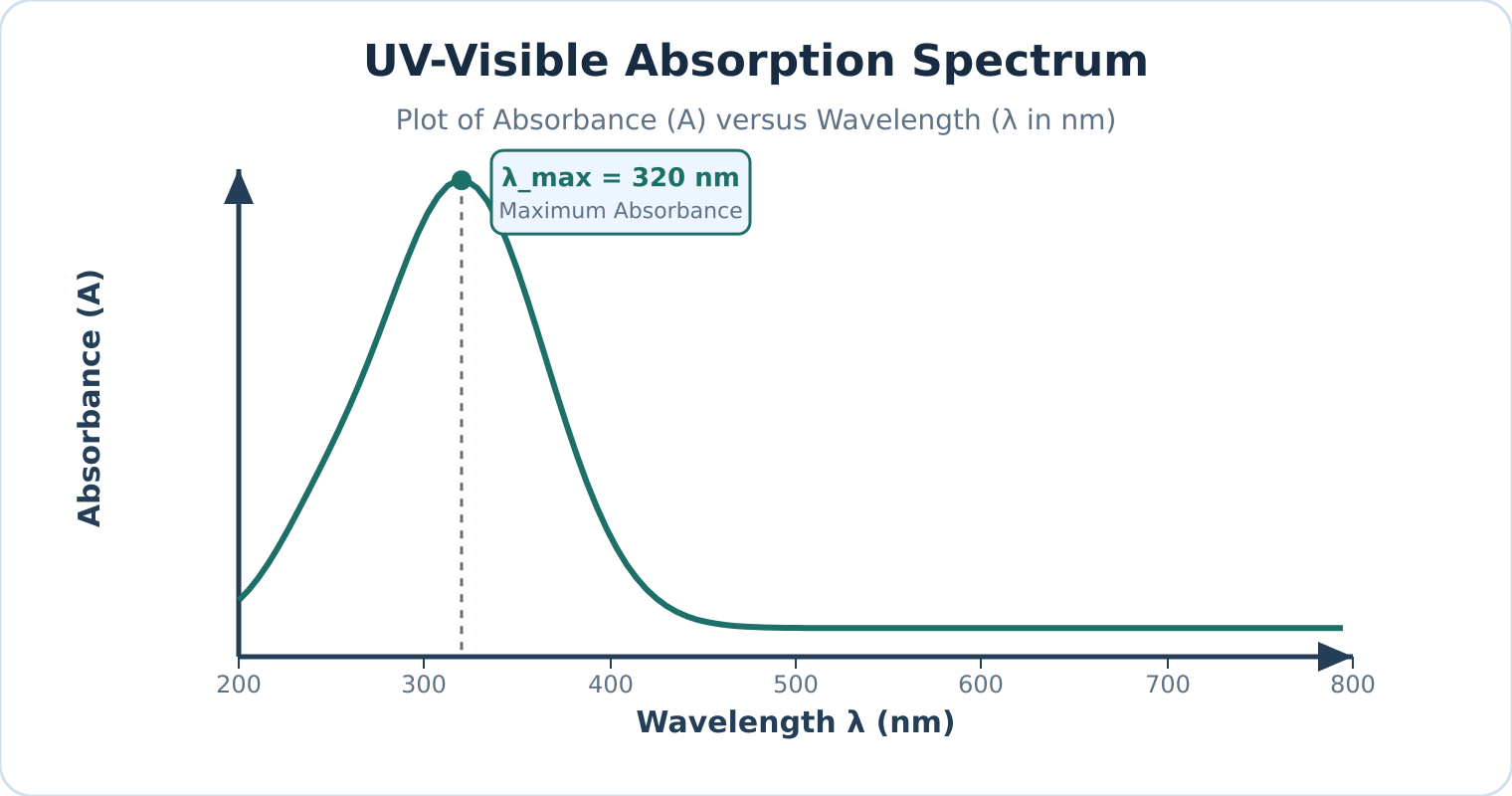
Figure: A representative UV–visible absorption spectrum plotting absorbance against wavelength, with peak absorption occurring at .
Instrument components
| Component | Materials & Types | Function & Operational Constraints |
|---|---|---|
| Radiation source | Deuterium () or Hydrogen () discharge lamps (UV: ); Tungsten–halogen filament lamp (Visible: ); Xenon flash lamp (UV–vis continuum) | Delivers stable, continuous radiation across the target spectral range. Gas discharge lamps generate light via an electric arc through gas rather than thermal incandescence. |
| Monochromator | Entrance slit; Collimating mirrors; Reflection diffraction grating or quartz prism; Exit slit | Spatially disperses polychromatic light into constituent wavelengths and isolates a narrow spectral bandwidth. |
| Beam splitter | Half-silvered beam splitting mirror; Rotating mirrored chopper disc | Directs monochromatic light alternately or concurrently through the reference and sample paths. Strict splitting is electronically calibrated against the baseline. |
| Sample & reference cells (cuvettes) | Fused quartz or synthetic silica (); Optical glass (); Disposable optical plastic (visible range only) | Holds solutions in a precision optical path (standard path length ). Cuvette optical faces must remain pristine, parallel, and chemically inert. |
| Detector | Photomultiplier tube (PMT); Silicon photodiode; Photodiode array (PDA) | Translates transmitted photons into an amplified electrical signal with high quantum efficiency, linear response, and rapid response times. |
Watch out. Always verify the cuvette material's operational wavelength cutoff. Standard optical glass and common plastics absorb strongly throughout the ultraviolet region (). Fused silica/quartz cuvettes are mandatory for UV measurements, although specialized UV-transparent disposable polymers can be used within strictly qualified solvent limits.
Reference blank and solvent selection
Reference blank
A reference blank is a matched reference cell filled with pure solvent and any background reagents (excluding the analyte) placed in the reference path to set the baseline intensity . Because cuvette windows reflect light and solvents scatter or slightly absorb radiation, the reference blank optically cancels these background contributions:
- Refractive index mismatches and reflection losses at cell interfaces are equalized.
- Non-analyte reagent and solvent absorbances are automatically subtracted.
UV cutoff wavelength
The UV cutoff wavelength is the specific wavelength threshold below which a pure solvent itself begins absorbing strongly (). To prevent total radiation attenuation and distorted readings, analysts must choose a solvent transparent across the analyte’s absorption bands:
- Water: Cutoff (ideal for aqueous analysis)
- Acetonitrile: Cutoff
- Cyclohexane / Hexane: Cutoff
- Methanol / Ethanol: Cutoff
- Chloroform: Cutoff
Watch out. UV–visible spectroscopy alone cannot provide definitive structural identification of an unknown compound. Because electronic transition bands are broad, UV–vis spectra primarily identify conjugated -electron systems and chromophores ( and ). Complementary methods like FTIR, NMR, and Mass Spectrometry are indispensable for full structural elucidation.
Applications of UV–visible spectroscopy
- Quantitative concentration analysis: Unknown concentrations of active ingredients, metal chelates, and biochemical analytes are quantified at using standard calibration curves governed by the Beer–Lambert law.
- Reaction kinetics: Progress of chemical and biochemical reactions is tracked in real-time by monitoring changes in absorbance over time () as reactants deplete or products evolve.
- Characterisation of dyes and pigments: Measurement of spectral absorption profiles and molar absorptivity () characterizes industrial dyes, organic indicators, and transition metal coordination complexes.
- Purity checking and quality control: Detection of trace UV-absorbing impurities in bulk solvents or pharmaceuticals (e.g., verifying the absence of toxic benzene impurities in absolute ethanol or cyclohexane).
- Conjugation and structural probes: Evaluation of bathochromic (red) and hypsochromic (blue) shifts reveals the degree of -conjugation, steric hindrance, and solvent polarity effects.
- Colorimetric clinical assays: Analytes lacking native UV–vis absorption (such as glucose, urea, or cholesterol) are coupled with specific enzymatic or chromogenic reagents to generate intensely colored chromophores suitable for photometric quantification.
Self-check questions
-
Why are deuterium lamps called discharge lamps rather than filament lamps?
Answer: Deuterium lamps generate radiation by striking a low-voltage electrical arc through pressurized deuterium gas, electronically exciting the gas molecules into a dissociated continuum state. In contrast, filament lamps pass current through a solid metal wire (such as tungsten) to generate light via thermal incandescence. -
What happens to the measured absorbance at a given wavelength if the analyte does not absorb light there ()?
Answer: When no radiation is absorbed by the analyte, the transmitted sample intensity equals the reference intensity (). Substituting this into the absorbance equation gives:The measured absorbance is zero, corresponding to transmittance ().
Infrared absorption and types of vibration
Working principle
Infrared spectroscopy
Infrared (IR) spectroscopy, also known as vibrational spectroscopy, studies the interaction of infrared radiation with matter. For ordinary molecular systems, mid-IR absorption probes quantized vibrational energy gaps rather than valence-electron excitations. When a molecule absorbs infrared radiation matching a resonant vibrational frequency, it transitions from a lower quantized vibrational level to a higher one (accompanied by rotational transitions in the gas phase).
Under the harmonic oscillator approximation, fundamental vibrational transitions obey the selection rule:
where is the vibrational quantum number (). Real molecular bonds exhibit anharmonicity, allowing weak overtone transitions () to appear at higher wavenumbers.
Although the broad infrared spectrum spans roughly to (classified into near-, mid-, and far-IR), standard chemical analysis utilizes the mid-infrared region, spanning to .
Condition for IR activity
Infrared activity
Infrared activity requires that the electric dipole moment of the molecule changes periodically during the vibration for an absorption band to appear:
where is the molecular dipole moment and is the normal coordinate of vibration.
Infrared radiation is an oscillating electromagnetic wave with an oscillating electric field. Energy transfer occurs only when the molecular motion produces an oscillating dipole of matching frequency to couple with the electric field of the radiation.
- Homonuclear diatomic molecules (, , , , ) maintain symmetrical electron distributions throughout their single stretching vibration. Because their dipole moment remains strictly zero at all internuclear distances (), they have no dipole-allowed fundamental absorption and are IR inactive.
- Heteronuclear diatomic molecules (, , , ) feature an asymmetric charge distribution. As the bond stretches and contracts, the dipole moment oscillates (), rendering the vibration IR active.
- Polyatomic molecules (, , , , ) possess multiple normal modes. IR activity is determined independently for each individual vibration.
Watch out. A molecule does not require a permanent dipole moment at equilibrium to show an IR spectrum, nor are all vibrational modes in a polyatomic molecule automatically active. For example, linear is nonpolar at equilibrium (), but its asymmetric stretching and bending modes induce a temporary oscillating dipole, making them IR active. Conversely, its symmetric stretch preserves centrosymmetry () and remains IR inactive.
IR spectrum structure
An infrared spectrum is conventionally plotted with percentage transmittance () on the vertical axis against wavenumber (, in ) on the horizontal axis, running from high wavenumber () on the left to low wavenumber () on the right.
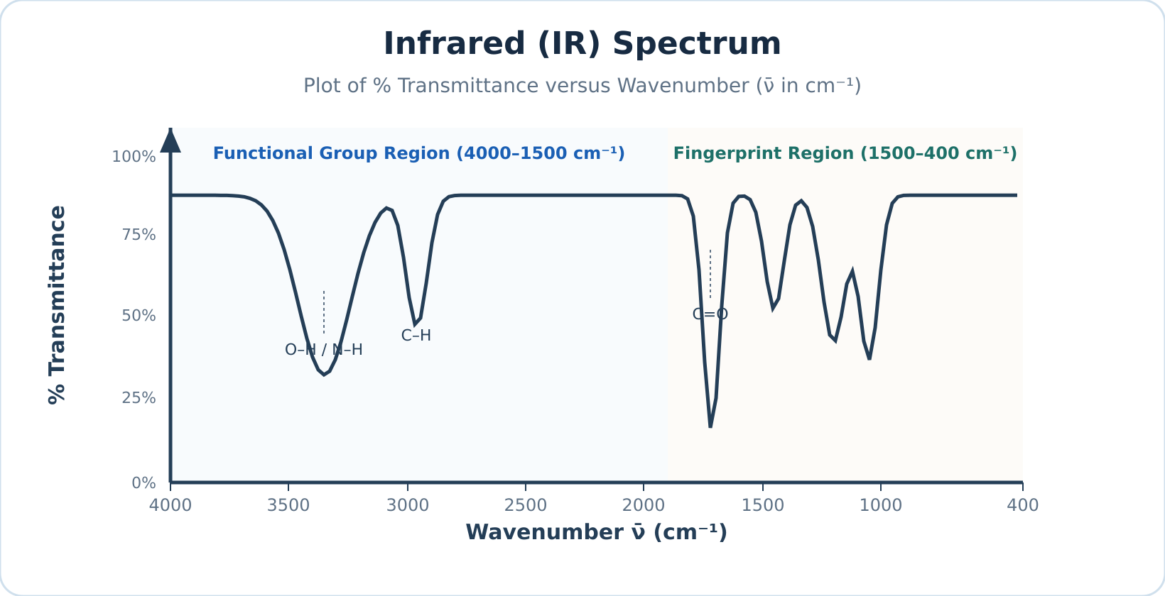
Figure: Schematic representation of an IR spectrum plotting percentage transmittance () against wavenumber (), where absorption bands appear as downward troughs.
At resonant frequencies where the molecule absorbs infrared radiation, less radiation reaches the detector, producing a downward trough in . (When plotted as absorbance , absorptions appear as upward peaks.)
The mid-IR spectrum is divided into two primary analytical zones:
- Functional group region (): Contains characteristic stretching absorptions of specific functional groups (such as , , , and ), which appear at relatively consistent positions regardless of the rest of the molecule.
- Fingerprint region (): Dominated by complex bending motions and single-bond skeleton stretches (, , ). This zone produces an intricate, unique pattern diagnostic of the specific molecule.
Types of molecular vibrations
Normal modes
In a polyatomic molecule, vibrations manifest as normal modes—coordinated atomic displacements oscillating at a characteristic frequency where all atoms pass through equilibrium simultaneously without translating or rotating the molecule as a whole. Complex modes can be categorized into stretching and bending motions.
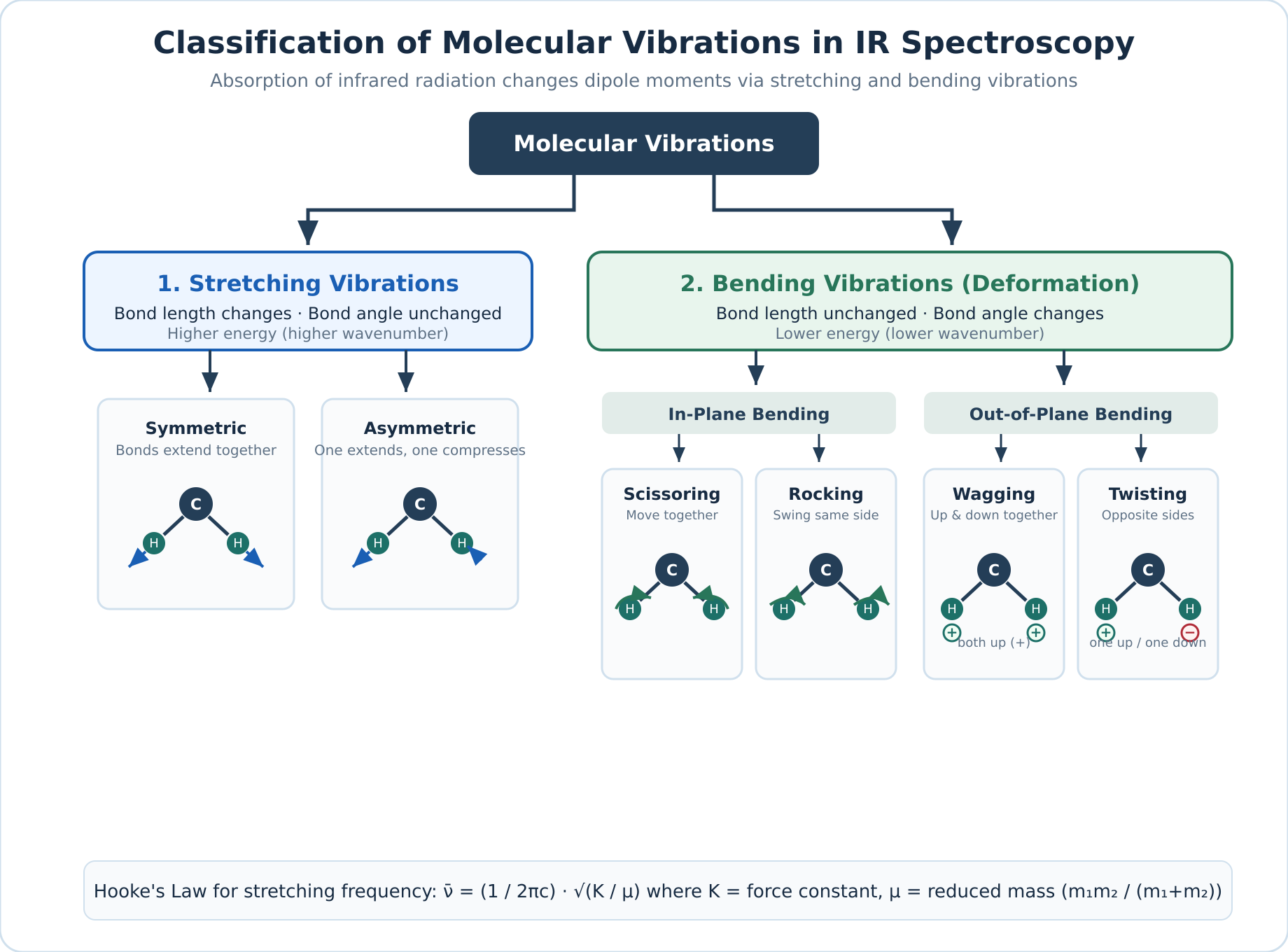
Figure: Classification of fundamental molecular vibrations into stretching and bending modes using a three-atom group.
| Mode | Subtype | Motion Plane | Atomic Displacement |
|---|---|---|---|
| Stretching | Symmetric | Along bond axis | Two or more bonds lengthen and contract simultaneously in phase. |
| Stretching | Asymmetric | Along bond axis | One bond lengthens while adjacent bonds simultaneously shorten. |
| Bending | Scissoring | In-plane | Two outer atoms move toward and away from each other, altering the bond angle. |
| Bending | Rocking | In-plane | The structural unit swings collectively back and forth within the molecular plane without changing the internal bond angle. |
| Bending | Wagging | Out-of-plane | Both outer atoms swing in unison to one side of the plane (+), then to the opposite side (). |
| Bending | Twisting | Out-of-plane | One outer atom swings above the plane (+) while the other swings below (), twisting around the central atom. |
Because stretching a chemical bond along its axis requires more energy than bending or deforming a bond angle, stretching vibrations consistently appear at higher wavenumbers than corresponding bending modes.
Self-check questions
-
Why is gas transparent to mid-infrared radiation whereas gas strongly absorbs it? Answer: is a homonuclear diatomic molecule whose dipole moment remains zero throughout bond stretching (), making it IR inactive. is heteronuclear, and stretching its polar bond changes its dipole moment (), making it IR active.
-
What is the difference between wagging and twisting vibrations? Answer: Both are out-of-plane bending vibrations, but in wagging both attached atoms move to the same side of the plane together, whereas in twisting one atom moves above the plane while the other moves below it.
Counting vibrations: carbon dioxide, water and HCN
Degrees of Freedom and Molecular Motion
Degrees of freedom
Degrees of freedom represent the number of independent coordinates required to specify the complete physical position and motion of every atom in a molecule. Every atom in a molecule can move along three mutually perpendicular Cartesian axes (, , and ). A molecule containing atoms therefore possesses a total of degrees of freedom describing all possible atomic motions in three-dimensional space.
These degrees of freedom partition into three distinct classes of motion:
- Translational motion: Shifting the entire molecule's centre of mass through three-dimensional space requires degrees of freedom (along the , , and axes) for all molecules.
- Rotational motion: Turning the entire molecule around its centre of mass depends strictly on molecular geometry:
- Linear molecules (such as , , or ) lie along a single axis. Rotation about the internuclear axis itself does not displace atomic nuclei and cannot be observed quantum mechanically, meaning it does not count as a degree of freedom. Only rotations about the two mutually perpendicular transverse axes displace atomic positions, giving rotational degrees of freedom.
- Non-linear molecules (such as or ) are not confined to a single straight line; rotation about any of the mutually perpendicular axes displaces the nuclei, yielding rotational degrees of freedom.
- Vibrational motion: The remaining degrees of freedom correspond to internal vibrations—periodic changes in bond lengths and bond angles. Subtracting translational and rotational motions from the total degrees yields the number of fundamental normal vibrational modes:
Here is the total number of atoms in the molecule (). Monatomic species (such as or , where ) possess only translational degrees of freedom and cannot undergo rotation or vibration.
Mode Counts and Observed IR Bands
Calculating or yields the number of independent normal vibrational coordinates, which does not necessarily equal the number of absorption peaks observed in an experimental infrared (IR) spectrum.
Infrared-inactive modes
Infrared-inactive modes are vibrational motions that produce no net change in dipole moment (). A vibrational mode absorbs an infrared photon only if the motion produces a periodic change in the molecule's net dipole moment. Highly symmetrical vibrations that leave the net dipole moment unchanged () are IR inactive and produce no absorption band.
Degenerate modes
Degenerate modes are two or more structurally distinct vibrational coordinates that possess the exact same vibrational frequency and energy. Because they absorb radiation at the exact same wavenumber, their absorption peaks coincide into a single observed fundamental band.
Non-fundamental transitions
Non-fundamental transitions are secondary vibrational absorptions arising from real anharmonic effects. Experimental spectra may feature additional weak absorption bands resulting from overtones (), combination bands (), difference bands, and rotational fine structure in gas-phase measurements.
Watch out. Do not assume that every calculated vibrational mode produces a separate peak in the IR spectrum. Always check each mode for a dipole moment change (IR activity) and check whether any active modes are degenerate (sharing the same wavenumber).
Worked Examples
Example 1: Counting fundamental vibrational modes across linear and non-linear molecules
Problem: Determine the molecular geometry, total degrees of freedom (), and number of fundamental vibrational modes for , , , , , methane (), benzene (), and cyclohexane (). State whether each molecule shows an IR spectrum.
Solution:
Count the total atoms in each chemical formula, identify whether the molecular framework is linear () or non-linear (), and check whether at least one vibration changes the dipole moment.
| Molecule | Formula | Total atoms () | Geometry | Total degrees () | Vibrational formula | Fundamental modes | Shows IR spectrum? |
|---|---|---|---|---|---|---|---|
| Hydrogen chloride | Linear | Yes (heteronuclear; changes) | |||||
| Nitrogen | Linear | No (homonuclear; always) | |||||
| Carbon dioxide | Linear | Yes ( of modes active) | |||||
| Hydrogen cyanide | Linear | Yes (all modes active) | |||||
| Water | Non-linear (bent) | Yes (all modes active) | |||||
| Methane | Non-linear (tetrahedral) | Yes (has modes that change the dipole moment) | |||||
| Benzene | Non-linear (planar ring) | Yes (has modes that change the dipole moment) | |||||
| Cyclohexane | Non-linear (puckered ring) | Yes (has modes that change the dipole moment) |
Example 2: Vibrational modes and IR activity of carbon dioxide ()
Problem: Calculate the number of fundamental vibrational modes for (), illustrate all modes, determine their IR activity, and explain how many fundamental absorption bands appear in an ideal harmonic IR spectrum.
Solution:
Carbon dioxide is a linear triatomic molecule () with a centre of inversion (centrosymmetric). In its equilibrium geometry, the two opposing bond dipoles cancel exactly, giving a net dipole moment .
The four normal vibrational modes are:
- Symmetric stretching (): Both oxygen atoms move simultaneously away from and toward the stationary central carbon atom along the molecular axis. Because both bonds lengthen and shorten equally at the same instant, the two bond dipoles always cancel out (). Therefore, the symmetric stretch is IR inactive.
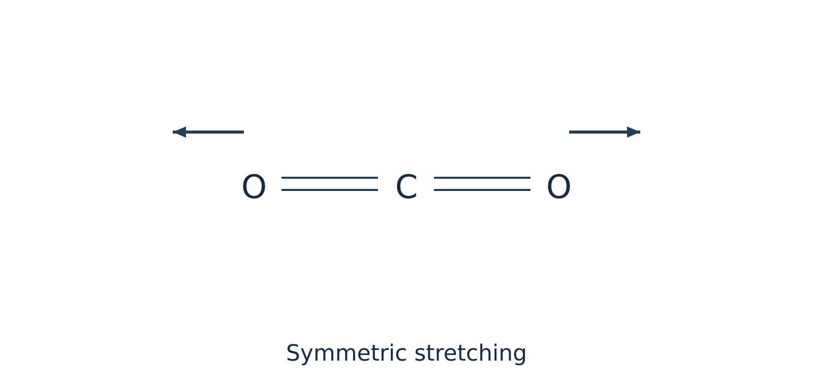 Figure 1: Symmetric stretching of preserves centrosymmetry () and is IR inactive.
- Asymmetric stretching (): One bond compresses while the other bond stretches. This breaks the symmetry of the charge distribution and produces a periodic oscillation in the net dipole moment along the bond axis (). Therefore, the asymmetric stretch is IR active.
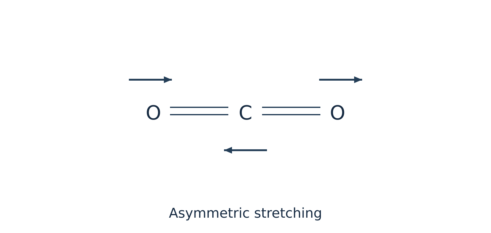 Figure 2: Asymmetric stretching of creates a net oscillating dipole moment () and is IR active.
- In-plane bending (): The two oxygen atoms move upward within the plane of the page while the carbon atom moves downward (and vice versa), deforming the bond angle. Because the bond dipoles no longer point in exactly opposite directions, a net dipole moment develops perpendicular to the molecular axis (). This mode is IR active.
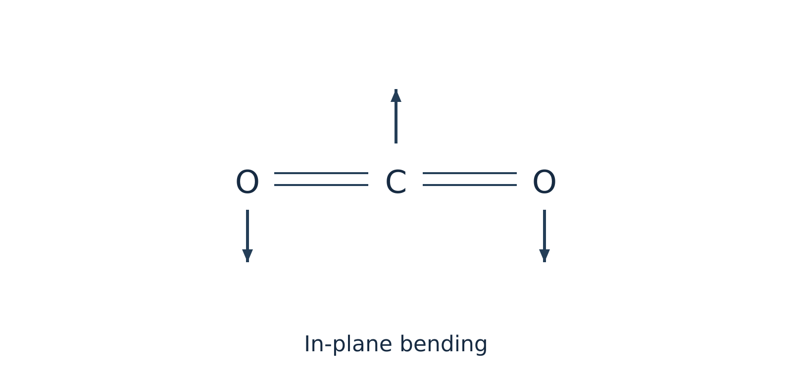 Figure 3: In-plane bending of induces a dipole moment perpendicular to the bond axis and is IR active.
- Out-of-plane bending (): The atoms bend in a plane perpendicular to the page (toward and away from the viewer). Exactly like the in-plane bend, this motion breaks linearity and creates an oscillating dipole moment (), making the mode IR active.
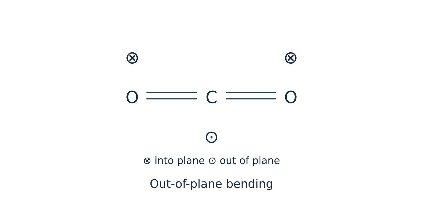 Figure 4: Out-of-plane bending of is also IR active and is degenerate with the in-plane bend.
Watch out. Do not label the out-of-plane bend of as IR inactive. Both the in-plane and out-of-plane bending modes produce a dipole moment change and are IR active; only one bending band appears around because the two modes are degenerate, not because one is inactive.
Summary for : Out of vibrational modes, vibrational coordinates are IR active (asymmetric stretch + two bends). Because the in-plane and out-of-plane bends differ only by a rotation around the molecular axis, they are doubly degenerate and absorb at the exact same wavenumber (). Thus, an ideal isolated harmonic molecule shows only fundamental absorption bands ( and ).
Example 3: Vibrational modes of water () and comparison with
Problem: Determine the fundamental vibrational modes and IR activity for bent water () and linear hydrogen cyanide (), and state the number of fundamental IR bands for each.
Solution:
Part A: Water ()
Water is a non-linear (bent) triatomic molecule (, bond angle ) with a permanent dipole moment.
- Symmetric stretching ( in isolated gas phase): Both bonds stretch and compress simultaneously in phase. Because the molecule is bent, changing both bond lengths alters the magnitude of the resultant dipole vector (). Thus, it is IR active.
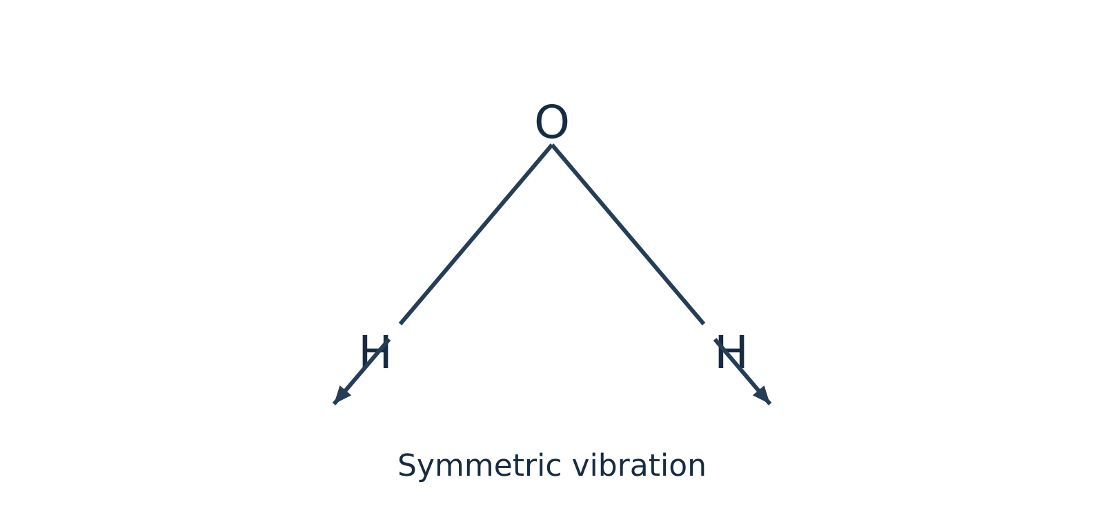 Figure 5: Symmetric stretching of bent changes the magnitude of the net dipole moment and is IR active.
- Asymmetric stretching ( in isolated gas phase): One bond lengthens while the other shortens, tilting the direction of the net dipole moment (). Thus, it is IR active.
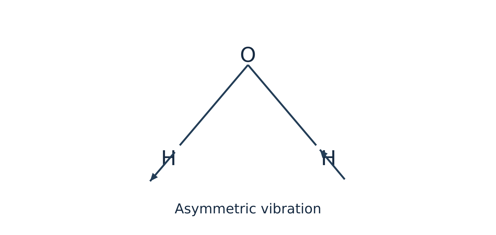 Figure 6: Asymmetric stretching of oscillates the dipole direction and is IR active.
- In-plane bending / scissoring ( in isolated gas phase): The bond angle opens and closes within the molecular plane, changing the net dipole magnitude (). Thus, it is IR active.
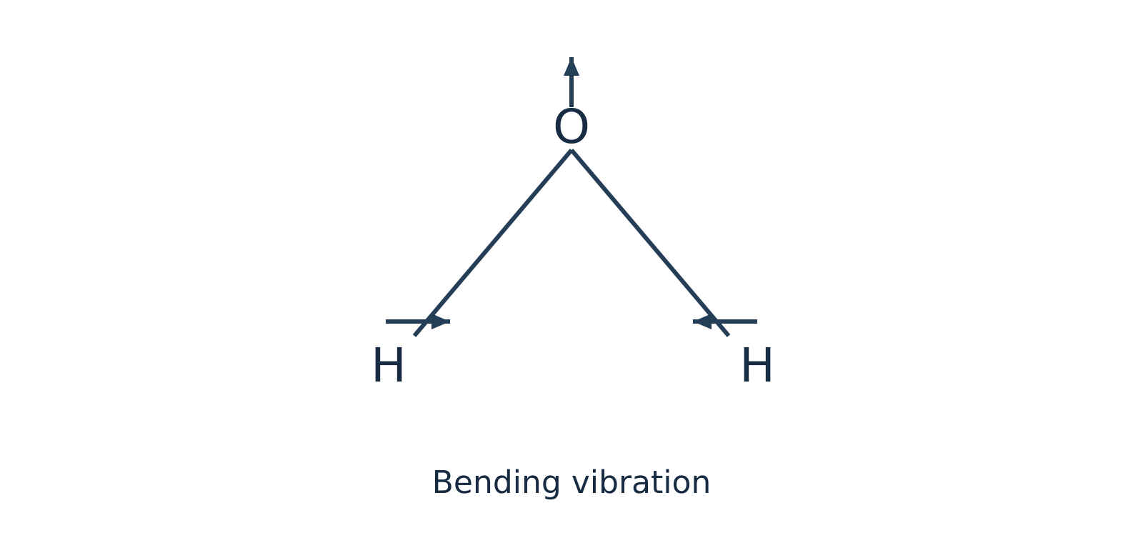 Figure 7: In-plane bending (scissoring) of alters the bond angle and dipole magnitude, making it IR active.
All modes of isolated gaseous are non-degenerate and IR active, giving distinct fundamental bands (note that in liquid water, intermolecular hydrogen bonding broadens and shifts these bands significantly).
Part B: Contrast with Hydrogen Cyanide ()
Like , is a linear triatomic molecule (), so it has fundamental vibrational modes: two stretching modes (predominantly stretch and stretch) and two perpendicular bending modes (in-plane and out-of-plane).
However, unlike centrosymmetric , is non-centrosymmetric because hydrogen and nitrogen are different atoms. Consequently:
- Both stretching modes change the dipole moment along the bond axis ().
- Both bending modes change the dipole moment perpendicular to the axis ().
Therefore, all vibrational coordinates are IR active in . Because the two perpendicular bends are doubly degenerate, exhibits fundamental absorption frequencies in its IR spectrum.
Self-Check Questions
-
Question: Acetylene () is a linear molecule and ammonia () is a pyramidal (non-linear) molecule. How many fundamental vibrational modes does each possess?
Answer: Both contain atoms. Linear has fundamental modes. Non-linear has fundamental modes. -
Question: Why is the symmetric stretching vibration IR inactive in but IR active in ? How do the two stretching modes of differ?
Answer: is linear and centrosymmetric, so equal stretching of both opposing bonds cancels the bond dipoles at every point (). is bent (the vector sum of bond dipoles changes magnitude during symmetric stretch), making it active. has two coupled stretching modes (predominantly and stretches); because it lacks a centre of symmetry, both stretching modes alter its dipole moment and are IR active. Symmetric and asymmetric descriptions are primarily applicable when terminal groups are identical.
Bond vibrations and force-constant calculations
Harmonic oscillator model
To determine the vibrational frequency of a chemical bond, two bonded atoms are modeled as masses ( and ) connected by a weightless spring. When displaced from their equilibrium distance, Hooke's law governs the restoring force pulling the atoms back toward equilibrium.
Force constant ()
Force constant is a measure of the stiffness of the chemical bond, representing the curvature of the potential energy curve near its equilibrium position. A larger force constant indicates a stiffer, more rigid bond.
Reduced mass ()
Reduced mass represents the effective inertial mass of a two-particle oscillating system vibrating along its internuclear axis, calculated as:
where and are the individual atomic masses in kilograms (). Because atomic weights are typically given in atomic mass units (), values must be converted to SI units using .
The classical vibrational frequency (, in or ) of this simple harmonic oscillator is:
Wavenumber ()
Wavenumber is the number of waves per unit length, defined as . Dividing the frequency expression by the speed of light () yields the fundamental infrared wavenumber equation:
Rearranging for the force constant () gives:
Watch out. Never mix centimetre and metre units in the force-constant formula. If you use the SI speed of light and reduced mass in to obtain in (equivalent to ), you must convert the wavenumber from to by multiplying by : . Alternatively, you may keep in only if you express the speed of light as .
Factors governing vibrational wavenumbers
The relationship demonstrates that the position of an infrared absorption band depends on two key physical variables:
- Bond strength (force constant, ): The vibrational wavenumber is directly proportional to . Stronger bonds possess greater stiffness (larger ) and require higher-energy photons to excite vibrations. For instance, across carbon–carbon bonds, the reduced mass remains identical ( for ), but as bond order increases from single () to double () to triple (), the force constant increases, shifting the stretching absorption progressively higher.
- Atomic masses (reduced mass, ): The vibrational wavenumber is inversely proportional to . Bonds involving light atoms (such as hydrogen, where ) absorb at high wavenumbers (), whereas bonds between heavy atoms absorb in the far lower wavenumber region.
| Bond comparison | Physical parameter altered | Effect on vibrational wavenumber () |
|---|---|---|
| Bond order: | is constant; force constant increases with bond order | increases () |
| Atom identity: vs | differs; increases sharply from to | drops markedly for the heavier bond |
| Isotopic substitution: vs | is unchanged (same electronic structure); increases | decreases for the heavier isotope () |
Localized group frequencies
In a polyatomic molecule (e.g., or ), vibrations are strictly coupled normal modes. However, when a functional group (such as or ) possesses a force constant or atomic mass substantially different from the rest of the molecular framework, the vibration remains largely localized. In these cases, the diatomic reduced-mass approximation provides reliable quantitative estimates.
Worked examples
Example 1: Force constant of carbon monoxide ()
Problem: A carbon monoxide () molecule absorbs infrared radiation at a wavenumber of . Calculate the force constant of the bond, given atomic masses and ().
Solution:
-
Calculate the reduced mass () in kilograms:
Converting to SI units:
-
Convert the wavenumber () to :
-
Compute the force constant (): Using and :
Example 2: Force constant of hydrogen chloride ()
Problem: Calculate the force constant of the bond given an experimental IR absorption input of , using approximate atomic masses and ().
Note: The supplied wavenumber is an exercise input, not a reference value for the observed HCl fundamental.
Solution:
-
Calculate the reduced mass () in kilograms:
Converting to SI units:
-
Convert the wavenumber () to :
-
Compute the force constant ():
Self-check questions
-
Question: How does infrared spectroscopy distinguish between a single bond and a double bond when both systems have the same reduced mass ()?
Answer: While is identical (), the double bond contains four shared electrons compared to two in the single bond, yielding a substantially larger force constant (). Because , the bond absorbs at a noticeably higher wavenumber () than the single bond (). -
Question (Illustrative isotopic shift): Assuming isotopic substitution leaves the electronic bond force constant unaffected, estimate the frequency ratio using integer masses , , and .
Answer:Because is constant:
Thus, deuterated hydrogen chloride absorbs at approximately times the wavenumber of standard .
Reading IR spectra and studying hydrogen bonding
Infrared spectroscopy
Infrared (IR) spectroscopy is one of the fastest laboratory techniques for identifying organic functional groups and probing non-covalent interactions. While local diatomic approximations treat bonds via their reduced mass () and force constant (), coupled polyatomic normal modes also give rise to characteristic absorption bands within predictable wavenumber () ranges.
Functional group and fingerprint regions
An infrared spectrum is traditionally divided into two diagnostic zones:
- Functional group region (): Contains relatively few, well-defined absorption bands arising primarily from stretching vibrations of key functional bonds, such as , , , , , and .
- Fingerprint region (): Contains a complex pattern of coupled single-bond stretches (, , ) and bending vibrations. Because this dense vibrational pattern is unique to the overall molecular skeleton, matching both the functional group region and the fingerprint region against an authentic reference standard recorded under identical conditions provides conclusive proof of identity.
Characteristic IR stretching frequencies
Under the harmonic oscillator model governed by Hooke's law, atomic masses and bond strengths directly dictate vibrational frequency:
where:
- is the wavenumber ()
- is the speed of light ()
- is the bond force constant ()
- is the reduced mass ()
When comparing carbon–carbon bonds of increasing order (, , and ), the reduced mass remains identical, but the force constant increases substantially. Consequently, stretching absorption shifts progressively toward higher wavenumbers:
Conversely, bonds involving light hydrogen atoms possess an exceptionally small reduced mass , shifting , , and fundamental stretches to high wavenumbers ().
| Functional group / bond | Approximate wavenumber () | Typical band shape and notes |
|---|---|---|
| Free (alcohol/phenol, dilute) | Sharp, medium-to-strong intensity | |
| Hydrogen-bonded (alcohol/phenol) | Broad, strong intensity | |
| Carboxylic acid | Very broad, diagnostic envelope overlapping the region | |
| Amine / amide | Medium intensity; primary amines typically display two distinct peaks | |
| Alkane | Medium-to-strong, located just below | |
| Alkene / aromatic | Medium intensity, located just above | |
| Terminal alkyne | Sharp, strong intensity | |
| Alkyne | Typically weak; absent if centrosymmetric symmetry prevents dipole change | |
| Carbonyl (general) | Very strong and sharp; amides near , ketones/aldehydes/esters near | |
| Alkene | Weak-to-medium; absent if symmetric geometry forbids dipole alteration |
Watch out. Do not assume every stretch appears above or that an absorption near always indicates an alkene. Resonance delocalisation in amides lowers the carbonyl bond order, shifting the stretch down to roughly , directly overlapping the region. Always evaluate peak intensity (carbonyls are intensely polar and absorb strongly) and companion bands (such as or ester stretches) before finalizing assignments.
Studying hydrogen bonding by IR spectroscopy
Hydrogen bonding
Hydrogen bonding occurs when a hydrogen atom covalently bonded to an electronegative donor ( or ) interacts electrostatically with an unshared lone pair on an electronegative acceptor ( or ). This non-covalent interaction withdraws electron density from the covalent donor bond, lengthening and weakening it.
Because the covalent bond force constant decreases, the stretching absorption shifts to a lower wavenumber. Furthermore, because condensed phases exhibit a statistical distribution of hydrogen-bond distances and orientations, the resulting peak broadens significantly into a wide band ().
IR dilution experiments conducted in a non-polar, non-hydrogen-bonding solvent (such as ) distinguish between two primary modes:
-
Intermolecular hydrogen bonding: Occurs between separate, independent molecules. In p-nitrophenol (), the and groups occupy opposite ends of the rigid aromatic ring (-positions) and cannot interact internally. Instead, intermolecular networks assemble: In concentrated solutions, p-nitrophenol displays a broad absorption band near . Upon progressive dilution with an inert solvent, the solvent isolates individual solute molecules, disrupting intermolecular hydrogen bonds. Consequently, the broad associate band weakens and a sharp free band emerges at a higher wavenumber ().
-
Intramolecular hydrogen bonding: Occurs between proximate functional groups within the same molecule when stereochemistry permits a stable five- or six-membered chelate ring. In o-nitrophenol (), the adjacent () hydrogen and oxygen form an internal six-membered ring. Because this interaction is an internal molecular feature, diluting the sample in an inert solvent does not disrupt the chelate ring. The shifted stretching band () remains essentially invariant with respect to concentration (though strong temperature shifts or coordinating polar solvents can disrupt it).
Watch out. Avoid using catechol (benzene-1,2-diol) and hydroquinone (benzene-1,4-diol) as ideal contrasts for dilution experiments. While catechol establishes an intramolecular hydrogen bond via one hydroxyl group, its second group remains free to form intermolecular associates at elevated concentrations. Comparing o-nitrophenol with p-nitrophenol provides an unambiguous, textbook contrast.
Example 1: Distinguishing isomers using IR dilution
Problem: Spectra of two nitrophenol isomers are measured across a concentration gradient in an identical non-hydrogen-bonding solvent at constant temperature. One sample exhibits an emerging, high-wavenumber free band upon progressive dilution, whereas the other sample retains its hydrogen-bonded band position without concentration-dependent shifting. Explain the assignments.
Solution:
- Differentiate concentration from association effects: Evaluate band shapes and peak positions rather than raw absorbance values alone, since dilution universally reduces total absorbance per the Beer–Lambert law.
- Assign the concentration-dependent sample: The progressive emergence of a sharp, high-wavenumber free band reveals the dissociation of intermolecular hydrogen bonds as intermolecular spacing increases. This behavior confirms the sample is p-nitrophenol, which cannot form an internal chelate ring.
- Assign the concentration-independent sample: Invariance of the hydrogen-bonded absorption frequency upon dilution demonstrates an internal structural interaction unaffected by intermolecular distance. This confirms the sample is o-nitrophenol, which forms a stable six-membered intramolecular chelate ring.
- Cross-validate structural identity: Check the full fingerprint and functional group spectra against authentic reference libraries to verify overall consistency alongside the dilution response.
Other analytical applications of IR spectroscopy
- Checking sample purity: Pure compounds yield clean, reproducible absorption spectra with characteristic peak shapes. Extraneous bands that do not belong to the authentic reference spectrum (such as an unexpected sharp peak near in a purified secondary alcohol) clearly expose functional-group impurities. However, the absence of extraneous peaks indicates optical purity within detection thresholds, not absolute chemical purity.
- Monitoring reaction kinetics: Recording IR spectra at fixed time intervals enables quantitative tracking of reaction progress. For example, during the oxidation of a secondary alcohol to a ketone, the gradual decrease in absorbance of the broad band () accompanied by the simultaneous growth of the sharp carbonyl band () directly tracks conversion kinetics.
Self-check questions
-
Question: Why does hydrogen bonding shift the covalent stretching absorption to a lower wavenumber rather than a higher one?
Answer: Formation of a hydrogen bond () draws electron density toward the acceptor, lengthening and weakening the covalent bond. This decreases the effective force constant . Because vibrational wavenumber is directly proportional to the square root of the force constant (), a smaller force constant lowers the stretching frequency. -
Question: A sample displays a strong, sharp IR peak at alongside two medium-intensity bands at and . Why is assigning the band to an alkene stretch likely incorrect?
Answer: Amide carbonyl () stretching frequencies are shifted down to due to resonance delocalisation from the adjacent nitrogen lone pair, and primary amides characteristically display two stretching bands in the region. Furthermore, carbonyl stretches possess high dipole moments and yield very strong absorption bands, whereas alkene stretches are characteristically weak to medium in intensity.
Dielectric thermal analysis: principle, instrument and uses
Operating principle
Dielectric thermal analysis (DETA)
Dielectric thermal analysis (DETA), also designated as dielectric analysis (DEA), measures how the alternating-current (AC) dielectric response of a material changes with temperature, time, or frequency. It is widely used for polar and semi-polar materials such as polymers, thermosetting resins, adhesives, glasses, and ceramics.
When a sinusoidal AC voltage is applied across a sample placed between two electrodes, the alternating electric field interacts with two distinct microscopic species inside the material:
- Permanent molecular dipoles undergo dipolar relaxation, rotating to reorient with the alternating electric field.
- Mobile free ions (often trace impurities or catalyst residues) undergo ionic migration, drifting translationally toward the oppositely charged electrode.
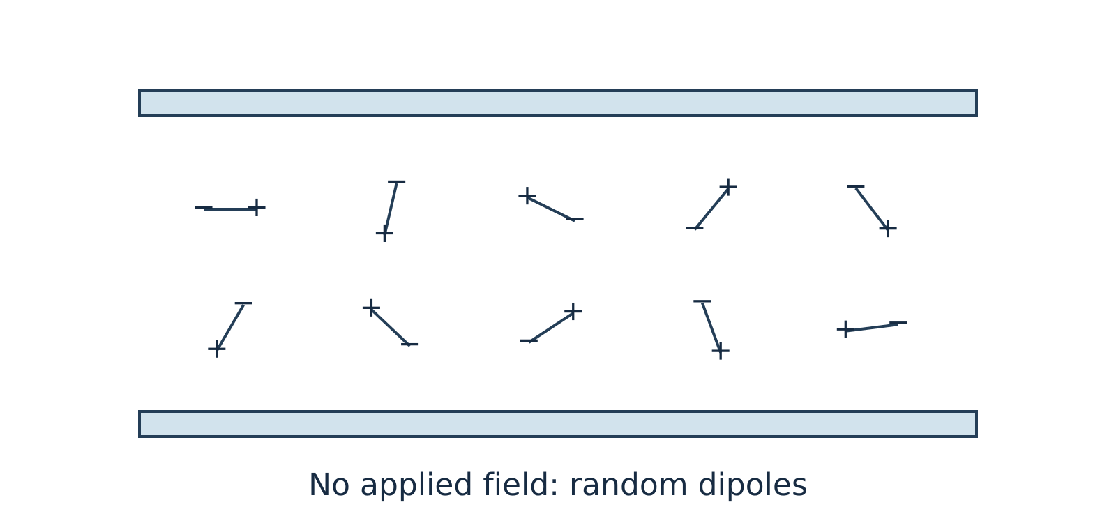
Figure 11.1: In the absence of an external electric field, thermal motion keeps molecular dipoles randomly oriented.
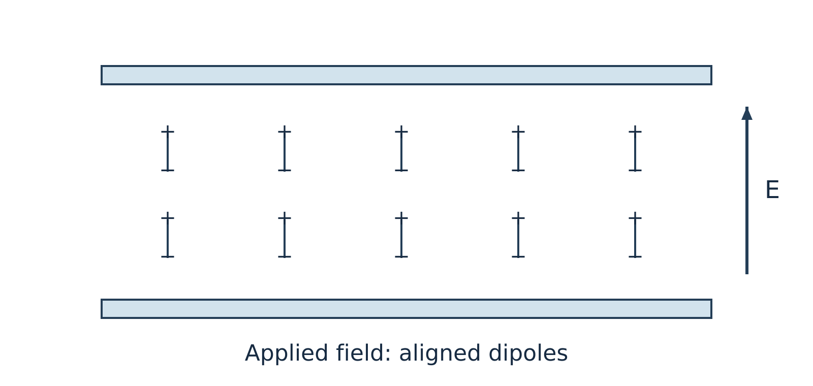
Figure 11.2: Under an applied electric field, dipoles experience torque and partially align with the field direction.
Watch out. Do not confuse ions with dipoles. Ions do not "align" in place, and bound dipoles do not migrate across the sample. Instead, dipoles rotate (orientation polarisation) while free ions drift toward opposite electrodes (ionic conduction). Furthermore, although static diagrams show neat alignment at a single instant, an AC field reverses continuously and thermal agitation opposes alignment, so dipoles never remain perfectly aligned.
Dipolar relaxation and ionic conduction impart both storage and loss components to the dielectric response. The analyser measures the current amplitude and its phase relative to the applied voltage to separate these components.
Dielectric parameters
Using the harmonic time convention , the dimensionless complex relative permittivity is expressed as:
Where:
- is the angular frequency (in )
- is the AC frequency (in )
For a parallel-plate cell of plate area and electrode separation , the measured capacitance is and the AC conductance is , where is the vacuum permittivity.
| Parameter | Symbol | Physical Meaning |
|---|---|---|
| Relative permittivity (storage permittivity) | Dimensionless measure of a material's ability to polarise and store electrical energy reversibly in an electric field. | |
| Dielectric loss factor | Dimensionless measure proportional to the electrical energy dissipated as heat per cycle due to viscous drag on rotating dipoles and migrating ions (not the energy itself). | |
| Loss tangent (dissipation factor) | Dimensionless ratio of loss factor to storage permittivity, where is the dielectric loss angle by which electric displacement lags the electric field. |
The dissipation factor is defined by:
Note that the loss angle is the complement of the current–voltage phase angle for the equivalent parallel capacitor–conductance model (), rather than the current–voltage phase shift itself.
Watch out. Student notes often state that a low makes a material a good thermal insulator. In reality, low is desired for electrical insulation and low-loss capacitors because it minimises dielectric heating under AC fields. Dielectric loss measurements do not measure thermal conductivity or guarantee thermal insulation.
Example 1: Calculating the dissipation factor (illustrative example)
Problem:
At a fixed frequency and temperature, a polymer film tested in a DETA cell has a relative storage permittivity and a dielectric loss factor . Assuming linear dielectric behaviour, calculate the dissipation factor .
Solution:
The dissipation factor is (dimensionless).
Instrumentation and working
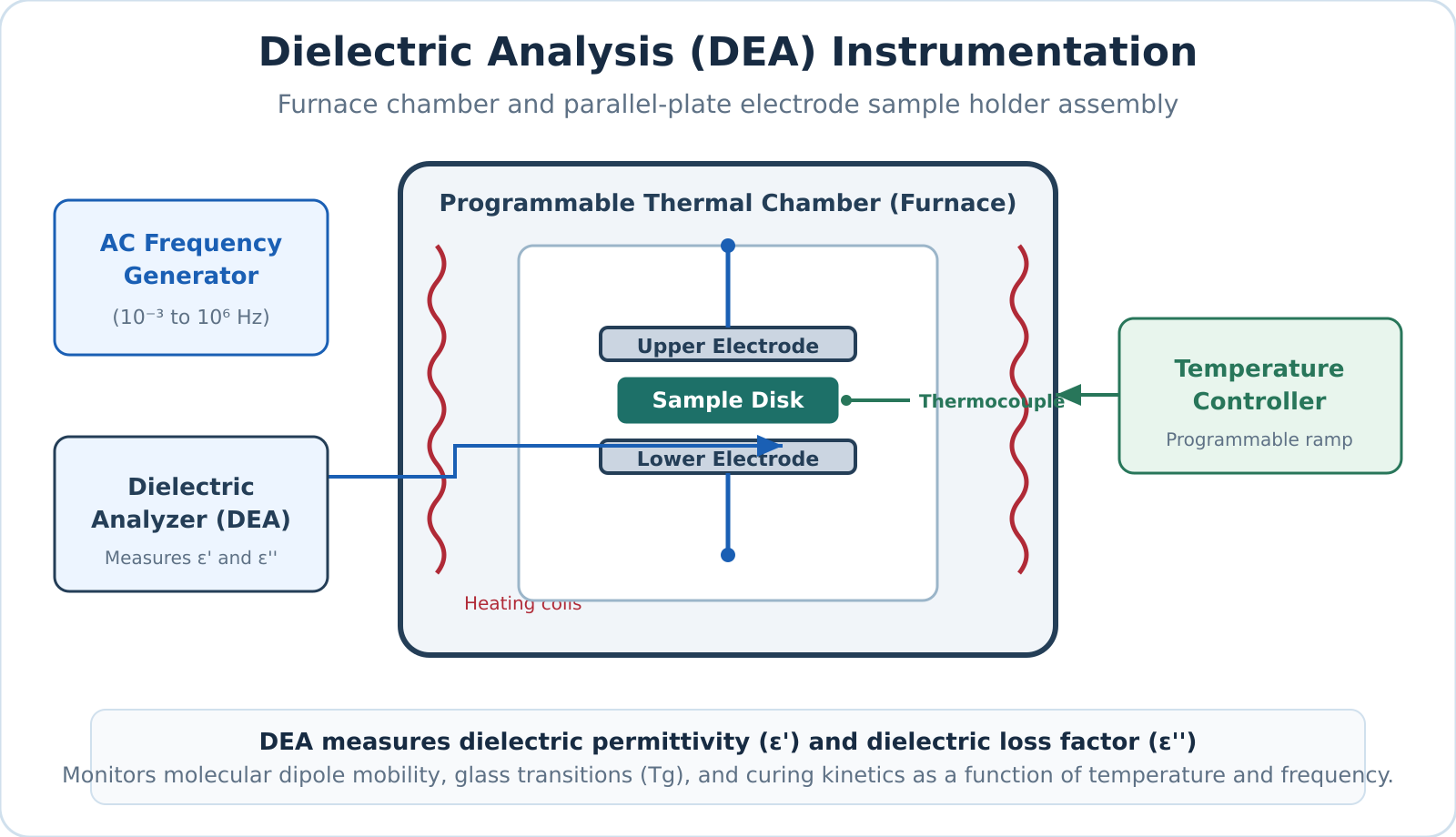
Figure 11.3: Schematic of a DETA setup showing the sample between electrodes inside a programmable furnace connected to a dielectric analyser.
A standard DETA instrument comprises the following primary components:
- Sample holder and electrodes: Parallel metal plates or interdigitated comb electrodes that directly contact the sample (thin film, liquid resin, powder, or pellet).
- Frequency generator (AC source): Delivers a sinusoidal voltage of known amplitude and selectable frequency (fixed or swept across multiple frequencies).
- Temperature-programmable furnace and controller: Heats, cools, or holds the sample isothermally at a controlled rate while preventing thermal overshoot.
- Temperature sensor (thermocouple or RTD): Positioned in close proximity to the sample to monitor its actual temperature accurately.
- Environmental control unit: Purges the furnace chamber with dry air or an inert gas such as nitrogen to prevent oxidative degradation or moisture absorption.
- Dielectric analyser and recorder: Measures the amplitude and phase of the resulting current relative to the applied voltage, calculates capacitance, conductance, , , and , and plots them as functions of temperature, time, or frequency.
Experimental procedure
- Mount the sample between the electrodes inside the furnace chamber and establish the required purge gas atmosphere.
- Apply a sinusoidal AC excitation voltage at one or more selected frequencies.
- Ramp or hold the furnace temperature according to a predetermined thermal program while continuously tracking sample temperature.
- Record , , and continuously as functions of temperature or curing time.
Applications of DETA
- Glass transition temperature () and relaxation processes: Segmental mobility changes near the glass transition produce a dispersion in storage permittivity () and pronounced peaks in the loss factor () when the molecular relaxation timescale matches the AC excitation frequency. Because dipole relaxation is a kinetic process, the apparent shifts to higher temperatures as measurement frequency increases.
- Curing of thermosetting resins and adhesives: During isothermal curing of epoxies or polyurethanes, crosslinking builds a rigid 3D polymer network that restricts ion drift and dipole reorientation. At constant temperature, ionic mobility drops and bulk resistivity rises significantly as curing progresses, allowing precise real-time tracking of gelation and vitrification.
- Moisture and quality monitoring: Because water has a very high dielectric constant ( at room temperature) and promotes ionic conduction, DETA sensitively detects trace moisture absorption, plasticiser loss, and batch-to-batch variations in polymers.
- Electrical insulation and capacitor development: Evaluating and over wide operational temperature and frequency ranges enables engineers to design low-loss dielectric films for capacitors and high-voltage electrical insulation.
Self-check questions
-
Question: Why does a polymer show a peak in as it is heated through its glass transition temperature ?
Answer: A segmental relaxation produces a loss peak when its characteristic relaxation timescale matches the period of the applied AC field. The peak temperature depends on the test frequency and does not necessarily equal the glass transition temperature determined by other thermal methods (e.g., DSC). -
Question: How does increasing the crosslinking density during isothermal epoxy curing affect ionic migration in a DETA experiment?
Answer: Crosslinking increases network tightness and local steric hindrance, which significantly reduces ionic mobility and causes the bulk electrical resistivity to rise.
Scanning electron microscopy: signals, instrument and uses
Scanning electron microscopy
Scanning electron microscopy (SEM) is a high-resolution imaging technique that visualizes solid specimen surfaces by sweeping a focused beam of high-energy electrons across a sample in a rectangular raster pattern. Unlike an optical microscope that focuses light using glass lenses, or a transmission electron microscope (TEM) that relies on electrons transmitted through an ultra-thin sample, an SEM detects signals emitted from the sample surface and maps their intensity coordinate-by-coordinate to display pixel brightness.
Electron–sample interactions and signals
When primary beam electrons penetrate a solid target, they undergo multiple elastic and inelastic scattering events within a pear-shaped interaction volume. The depth and geometry of this interaction volume depend on the incident beam energy and the average atomic number of the material, generating several distinct, detectable signals.
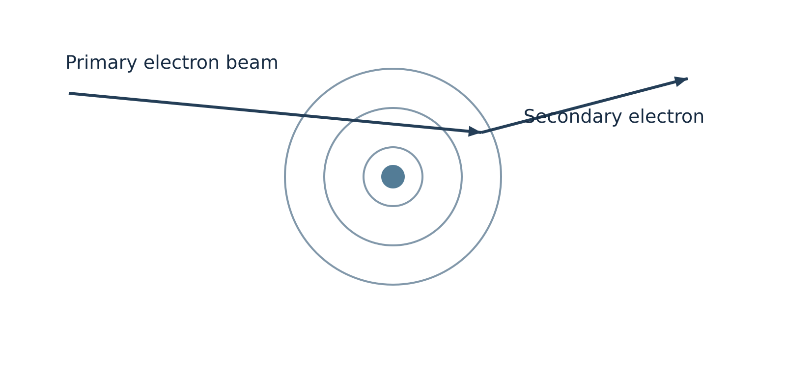
Figure 12.1: Inelastic collision ejecting a low-energy secondary electron.
Secondary electrons
Secondary electrons (SE) are ejected when primary beam electrons transfer a portion of their kinetic energy to atomic electrons via inelastic collisions, freeing loosely bound outer-shell electrons. Because secondary electrons have very low kinetic energies (typically below ), only those generated within a few nanometres of the surface can escape into the vacuum. The escape yield is strongly governed by local surface tilt, curvature, and edges, making secondary electron imaging the primary operational mode for revealing high-resolution surface topography, morphology, and texture.
Backscattered electrons
Backscattered electrons (BSE) are incident primary electrons deflected backward out of the specimen at large angles through predominantly elastic collisions with atomic nuclei. They retain a significant fraction of their initial primary beam energy and escape from deeper within the interaction volume than secondary electrons. Because heavier atomic nuclei (higher atomic number, ) possess a greater positive nuclear charge, they deflect electrons backward much more effectively. Regions of higher average yield more backscattered electrons and appear brighter under identical detector conditions, providing compositional (-contrast) alongside macro-topography.
Characteristic X-rays
Characteristic X-rays are emitted when an energetic beam electron ejects an inner-shell electron, and an electron from a higher orbital drops into the vacancy, releasing an X-ray photon with an energy precisely equal to the quantum difference between the two shells. Because these energy levels are unique to each element, coupling an SEM with an Energy-Dispersive X-ray Spectroscopy (EDS) detector enables elemental identification and chemical mapping. Supplementary techniques, such as Electron Backscatter Diffraction (EBSD), can be paired with SEM to resolve crystallographic phase and orientation.
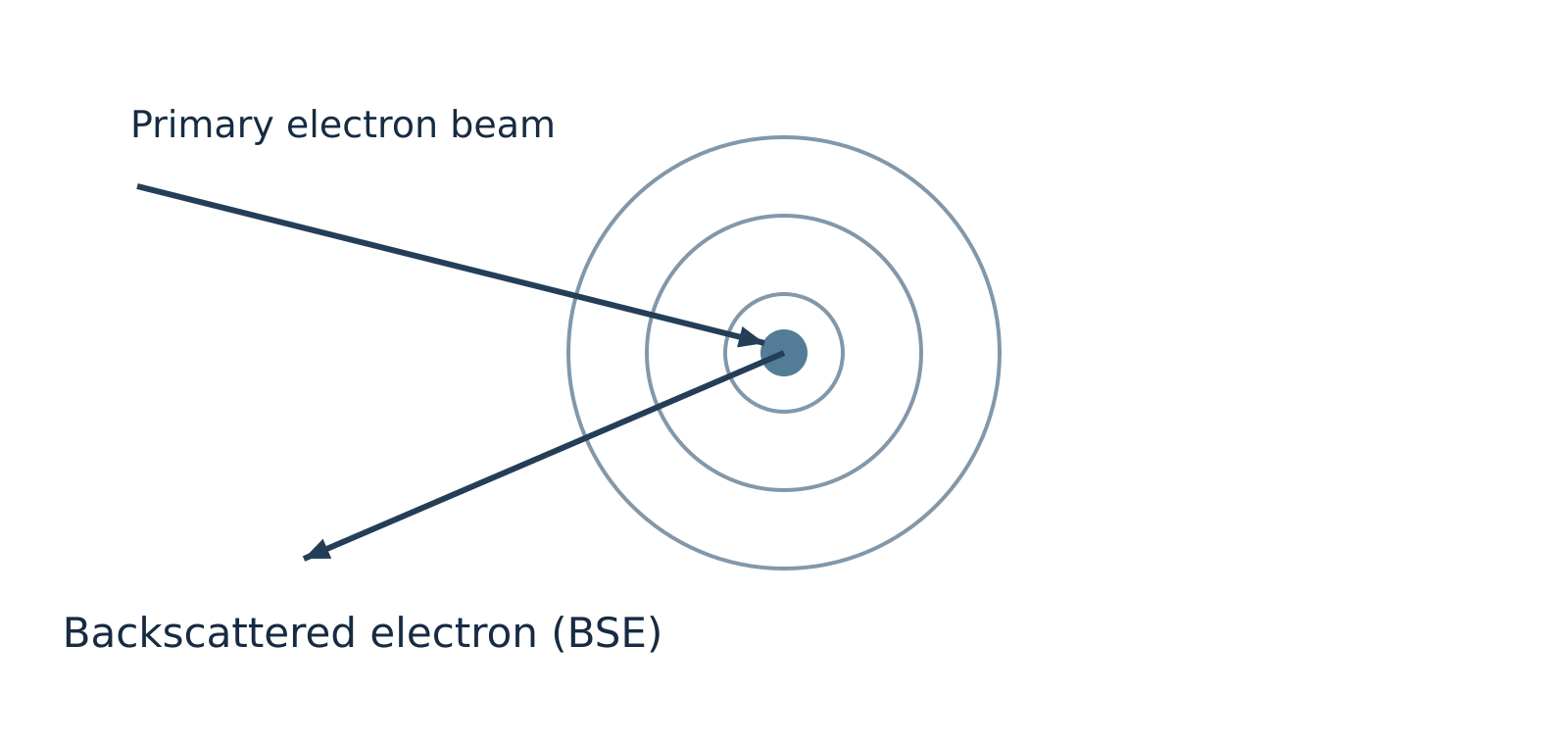
Figure 12.2: Elastic scattering of a primary electron by an atomic nucleus to produce a backscattered electron.
Watch out. Backscattered electrons originate predominantly from elastic nuclear scattering, not inelastic collisions. Furthermore, all elements backscatter electrons to some degree; higher- elements simply produce a higher backscatter yield rather than being the exclusive source of BSEs.
Comparison of emitted signals
| Signal | Origin / Mechanism | Escape Depth | Primary Information Provided |
|---|---|---|---|
| Secondary electrons (SE) | Inelastic ejection of outer-shell valence electrons | Very shallow (top few ) | Fine surface topography, morphology, and edge definition |
| Backscattered electrons (BSE) | Elastic nuclear deflection of incident beam electrons | Moderate (deeper sub-surface regions) | Compositional atomic-number () contrast and macro-topography |
| Characteristic X-rays | Inner-shell electron ionization followed by electronic relaxation | Deep interaction volume (micrometre scale) | Elemental identification and semi-quantitative chemical analysis (via EDS) |
Instrumentation and working
An SEM column operates under high vacuum () to prevent ambient gas molecules from scattering the electron beam, attenuating emitted signals, or degrading the electron gun filament.
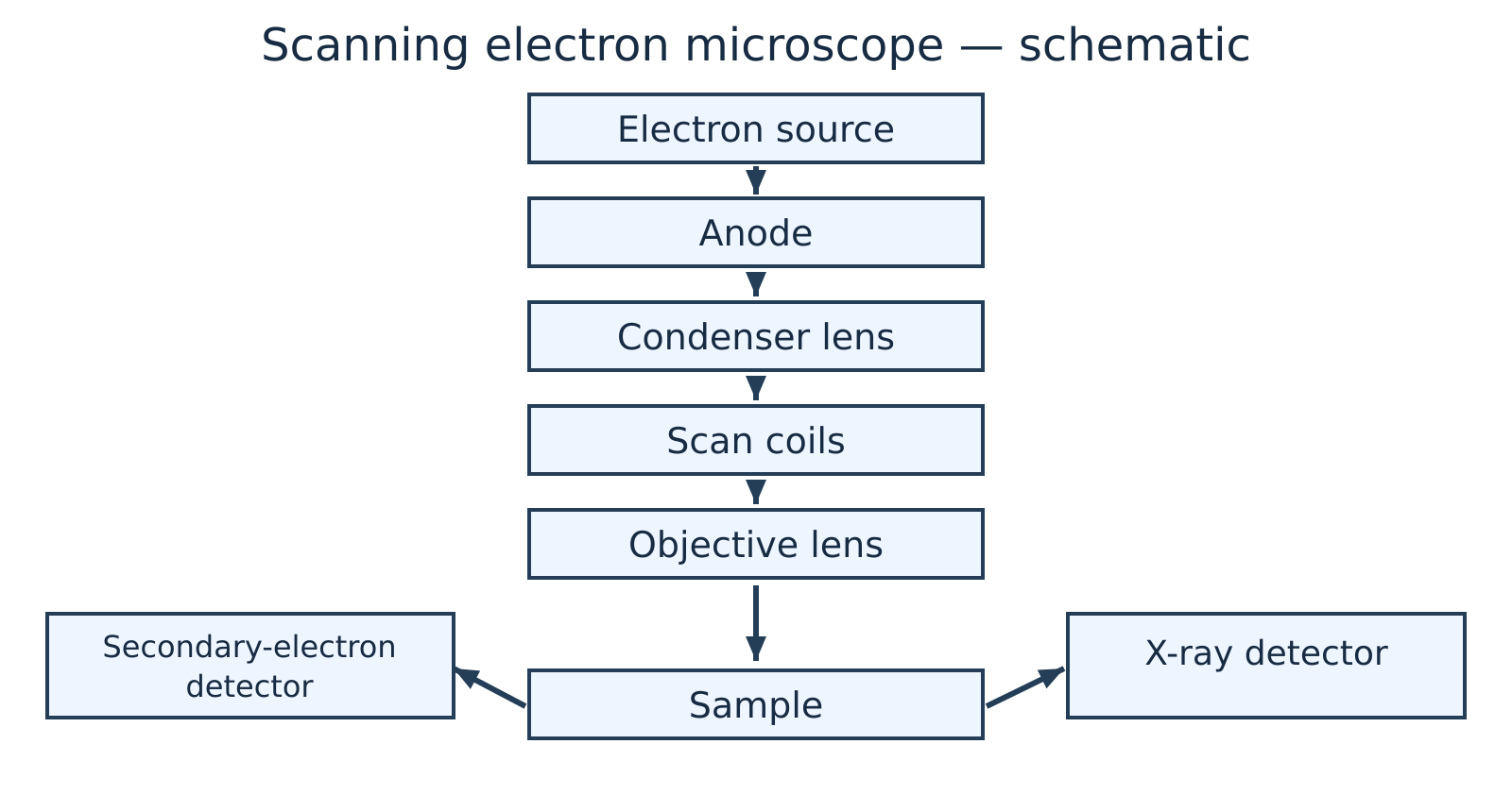
Figure 12.3: Schematic layout of a scanning electron microscope.
The primary components and operating sequence of an SEM include:
- Electron gun and anode: An electron source—such as a thermionic emitter (heated tungsten filament or crystal) or a field-emission gun (FEG)—generates free electrons. A high-voltage anode accelerates them down the column under an accelerating potential typically ranging from .
- Condenser lenses: One or more electromagnetic condenser lenses converge and demagnify the diverging electron stream, controlling the overall probe current reaching the specimen.
- Objective lens and aperture: The final electromagnetic lens focuses the demagnified electron beam into an extremely fine, nanometre-scale probe spot on the specimen surface.
- Scan coils: Deflection coils located within or above the objective lens sweep the focused electron beam synchronously across the sample surface in an raster pattern.
- Specimen stage and vacuum chamber: The specimen is mounted securely on a motorized, conductive stage inside an evacuated chamber, allowing precise multi-axis positioning (, tilt, and rotation).
- Detectors and signal processing: Specialized detectors—such as an Everhart–Thornley scintillator-photomultiplier detector for SEs, a solid-state annular diode for BSEs, and a silicon drift detector for EDS—collect emitted signals at each raster coordinate. The output current is amplified, digitized, and mapped as a corresponding greyscale pixel intensity on a display monitor.
Watch out. Due to the very narrow beam convergence angle, an SEM has a depth of field hundreds of times greater than that of an optical microscope, giving micrographs a pronounced three-dimensional appearance. However, standard SEM micrographs remain 2D intensity projections and do not provide direct mathematical 3D height (-coordinate) profiles without specialized stereoscopic or profilometric reconstruction.
Sample preparation and capabilities
Conductive coating
Under high vacuum, electrically insulating specimens accumulate negative surface charges from the incident beam, inducing bright glare streaks, beam deflection, and image distortion. Non-conducting samples are typically coated with an ultra-thin () conductive film of gold, platinum, or carbon via sputter deposition or thermal evaporation.
Environmental SEM
Environmental SEM (ESEM) and variable-pressure modes introduce a low-pressure gas environment into the chamber to naturally dissipate surface charge. This permits examination of uncoated or hydrated specimens when heavy-metal coatings could obscure fine nanoscale features or produce overlapping X-ray emission peaks during EDS analysis.
Specimen dehydration
Specimen dehydration is required under conventional high-vacuum SEM for biological and wet specimens. These samples undergo chemical fixation, critical-point drying, or cryo-fixation to prevent rapid outgassing, structural collapse, and chamber contamination.
Modern field-emission SEMs achieve sub-nanometre spatial resolution, continuously variable magnifications from up to over , and an exceptional depth of focus that keeps rough, non-planar surfaces in sharp focus across wide fields of view.
Example 1: Selecting SEM signal modes for failure analysis
Problem: A failure analysis engineer investigates a fractured steel fastener suspected of harbouring microscopic lead () inclusions distributed within a bulk iron () matrix, alongside sub-micrometre fatigue striations across the fracture surface. Which SEM operating mode should be selected to:
- Resolve the fine fatigue striations on the fracture ridges?
- Rapidly locate the dispersed heavy-metal inclusions?
- Confirm the elemental identity of the suspected inclusions?
Solution:
- Fatigue striation imaging (Secondary Electron mode): Secondary electrons escape only from the top few nanometres of the specimen surface and are exceptionally sensitive to micro-topographic variations and local tilt, providing sharp visual clarity of the fine fatigue striations.
- Inclusion screening (Backscattered Electron mode): The backscattered electron coefficient increases monotonically with atomic number (). Lead () scatters incident electrons far more effectively than iron (). Under BSE imaging, lead inclusions appear as bright, high-contrast features against a darker iron background.
- Elemental identification (Energy-Dispersive X-ray Spectroscopy): Positioning the focused electron probe directly over a bright inclusion and recording the emitted characteristic X-ray spectrum via EDS identifies the characteristic emission peaks (- and -series lines) of elemental lead.
Applications
- Materials science and metallurgy: Inspecting crystal grains, secondary precipitate phases, grain boundary segregation, corrosion pits, and differentiating between ductile dimple fracture and brittle cleavage surfaces.
- Microelectronics and nanotechnology: Measuring particle dimensions, agglomeration states, and aspect ratios of synthesized nanoparticles, as well as inspecting semiconductor wafers and interconnect lines for lithographic defects.
- Forensic and geological investigations: Characterizing microscopic gunshot residue (GSR) particles, identifying asbestos fibres, and analysing phase distributions in mineralogical thin sections.
- Biological and biomedical sciences: Examining surface structures of cells, bacteria, insect cuticles, biomaterial scaffolds, and dental implants.
Self-check questions
-
Question: Why do regions containing heavier elements appear noticeably brighter in a backscattered electron (BSE) image of a mechanically polished, flat cross-section? Answer: Heavier atomic nuclei have a higher positive nuclear charge (higher ), which exerts a much stronger Coulomb attractive force on passing beam electrons. This leads to a significantly higher probability of wide-angle elastic deflections, yielding a higher fraction of backscattered electrons collected by the detector.
-
Question: Why is an insulating ceramic specimen often coated with carbon instead of gold prior to qualitative and quantitative EDS analysis? Answer: Although both carbon and gold mitigate surface charging, gold produces strong characteristic - and -shell X-ray peaks that can overlap and mask characteristic peaks of common transition metals and light elements. Gold also exhibits higher X-ray absorption. Carbon introduces a single low-energy line (), leaving the rest of the analytical spectrum free from interference for heavier analytes.
Revision sheet and practice problems
Core Formulas and Unit Conventions
| Quantity / Law | Equation | Symbol Definitions and Standard Units |
|---|---|---|
| Photon energy | : Planck's constant (); : speed of light (); : wavelength (); : wavenumber () | |
| Transmittance | : incident light intensity; : transmitted light intensity ( is dimensionless; ) | |
| Absorbance | : absorbance (dimensionless) | |
| Beer–Lambert law | : molar concentration ( or ); : path length (); : molar absorptivity () | |
| Two-point concentration ratio | Valid for identical chemical species, wavelength, solvent, temperature, and cell path length | |
| Fundamental vibrational modes | <br> | : total number of atoms in the molecule |
| Reduced mass | : atomic masses. Convert to via multiplication by | |
| Harmonic vibrational wavenumber | : bond force constant (). For SI units: and | |
| Dielectric dissipation factor | : relative permittivity (dielectric storage); : dielectric loss factor ( is dimensionless) |
Watch out. Never mix centimetre wavenumbers () with the SI speed of light () when calculating force constants. Multiply in by to obtain before squaring.
Analytical Techniques Overview
| Technique | Probe / Perturbation | Physical Property Measured | Primary Analytical Information |
|---|---|---|---|
| UV–Visible Spectroscopy | UV–visible photons () | Electronic excitation absorbance ( vs ) | Conjugated -electron systems, chromophores, quantitative trace concentration () |
| Infrared (IR) Spectroscopy | Infrared radiation () | Vibrational resonant absorption ( vs ) | Characteristic functional groups, bond force constants (), intra- vs intermolecular H-bonding |
| Dielectric Thermal Analysis (DETA) | Alternating electric field across programmed temperature ramp | Complex permittivity (), dielectric loss factor (), vs | Dipolar and ionic relaxation dynamics, glass transition temperature (), polymer curing kinetics |
| Scanning Electron Microscopy (SEM) | Focused high-energy primary electron beam () | Secondary electrons (SE), backscattered electrons (BSE), characteristic X-rays | High-resolution surface topography (SE), compositional atomic-number contrast (BSE), elemental analysis (EDS) |
Rapid-Retrieval Questions
-
Why is Raman spectroscopy not an emission spectrum?
Raman spectroscopy measures the inelastic scattering of incident photons following an induced molecular polarization change, whereas emission spectroscopy measures radiation emitted when an electronically or vibrationally excited state spontaneously relaxes to a lower energy state. -
Can a colourless solution obey the Beer–Lambert law?
Yes. A solution appears colourless if it does not absorb in the visible spectrum (), but it may exhibit intense absorption in the ultraviolet region (). At an appropriate UV analytical wavelength (), it fully obeys the Beer–Lambert law under dilute conditions. -
What is the difference between a theoretically possible electronic transition and a symmetry-allowed transition?
Energy matching between molecular orbitals merely establishes that an excitation is energetically plausible. Quantum mechanical selection rules dictate whether the electric dipole transition moment integral is non-zero. Only symmetry-allowed transitions exhibit large molar absorptivities (); forbidden transitions appear extremely weak via vibronic coupling. -
Why is the IR activity criterion stated per vibrational mode rather than per molecule?
Molecules possess multiple degrees of vibrational freedom. A vibrational mode is IR active if and only if that specific coordinate displacement causes a net change in the molecular dipole moment (). Symmetrical molecules like possess both IR-active and IR-inactive modes simultaneously. -
Why does have fundamental vibrational modes, IR-active modes, but only fundamental IR absorption bands?
Linear () possesses fundamental modes:- Symmetric stretch: Non-polar; IR inactive ().
- Asymmetric stretch: Polar; IR active, giving an intense band at .
- Bending modes (2 orthogonal coordinates): Polar and IR active, but structurally and energetically degenerate, collapsing into a single absorption band at .
-
What is the role of the reference (blank) cell in a double-beam UV–visible spectrophotometer?
The reference cell contains pure solvent and all background reagents except the absorbing analyte. It automatically cancels out reflection losses, light scattering, and optical absorption from the solvent and cuvette walls across the wavelength scan. -
How does dilution in an inert solvent distinguish intermolecular from intramolecular hydrogen bonding in IR spectra?
Dilution in a non-polar solvent increases intermolecular separation, disrupting intermolecular hydrogen bonds and shifting broad associated bands () toward sharp, unassociated free stretching bands (). In contrast, intramolecular hydrogen-bonded chelates remain intact upon dilution, showing no spectral position shift. -
What does a low dissipation factor () indicate in DETA?
A low dissipation factor indicates that dielectric energy loss is minimal relative to stored capacitive energy (), demonstrating high electrical insulation efficiency, minimal dielectric heating, and low dielectric relaxation in the evaluated frequency and temperature domain. -
How do secondary electrons (SE) and backscattered electrons (BSE) differ in their physical origin in SEM?
- Secondary electrons (SE): Ejected from sample atoms following inelastic collisions with primary beam electrons; possess low kinetic energy () and originate within top surface layers (), yielding fine topographical contrast.
- Backscattered electrons (BSE): High-energy beam electrons deflected at large angles via elastic collisions with atomic nuclei; intensity scales with atomic number (), yielding compositional contrast.
-
Why can sample charging be a problem in SEM, and how is it managed?
Electrically insulating samples accumulate negative charges from the incident beam, deflecting subsequent electrons and producing severe image distortion, brightness artifacts, and astigmatism. It is managed by sputter-coating the specimen with an ultra-thin conductive metal layer (gold or platinum), grounding the sample stage, or operating in low-vacuum/environmental SEM mode.
Numerical Practice Problems
Problem 1: Absorbance from Percent Transmittance
A solution placed in a spectrophotometer shows a percentage transmittance of . Calculate its absorbance.
-
Convert percentage transmittance to fractional transmittance :
-
Apply the logarithmic relation between absorbance and transmittance:
Problem 2: Concentration Determination via Beer–Lambert Law
A solution exhibits an absorbance of in a cuvette of path length at a wavelength where the molar absorptivity is . Calculate the molar concentration of the solution.
-
Isolate concentration from the Beer–Lambert law ():
-
Substitute the given parameter values:
Problem 3: Two-Point Standard Ratio Analysis
A standard solution of a coloured complex with concentration gives an absorbance of at . Under identical experimental conditions and path length, an unknown solution of the same complex gives an absorbance of . Calculate the concentration of the unknown solution.
-
Establish proportionality between absorbance and concentration under identical cell parameters:
-
Calculate the unknown concentration :
Problem 4: Vibrational Degrees of Freedom
Calculate the total number of fundamental vibrational modes for:
- Linear carbon dioxide (, )
- Bent water (, )
-
Linear ():
-
Non-linear ():
Problem 5: Dielectric Dissipation Factor
During a DETA experiment at a fixed frequency and temperature, a polymer sample exhibits a relative permittivity and a dielectric loss factor . Calculate the dissipation factor ().
-
Apply the dissipation factor relation:
-
Substitute the measured dielectric parameters:
Long-Answer Practice Prompts
-
Beer–Lambert Law Derivation & Validation:
State the differential form of the Beer–Lambert law and integrate it to obtain . Sketch the standard calibration plot of versus , identify the physical meaning of its slope, and list four experimental prerequisites required for strict linear adherence. -
Electronic Excitations & Chromophore Conjugation:
Illustrate the four primary electronic transitions (, , , and ) on a molecular orbital energy-level diagram. Detail why extended conjugation in conjugated polyenes causes a bathochromic shift in . -
Double-Beam UV–Vis Spectrophotometry:
Draw a complete block diagram of a double-beam UV–visible spectrophotometer. State the specific function of the radiation sources, monochromator diffraction grating, quartz optical cells, rotating sector chopper, and photomultiplier tube detector. -
Infrared Selection Rules & Molecular Vibrations:
State the dipole-moment selection rule for fundamental infrared absorption. Illustrate the vibrational modes of and , classify each mode as IR active or inactive, and explain the exact number of observable fundamental IR absorption bands for both molecules. -
Hooke's Law & Bond Force Constants:
Express Hooke's law for diatomic harmonic vibrations relating , , and . Using this equation, explain the observed stretching frequency hierarchy across carbon–carbon bonds: -
Hydrogen Bonding Discrimination via IR Dilution:
Explain how infrared dilution analysis in an inert non-polar solvent distinguishes ortho-nitrophenol from para-nitrophenol. Provide supporting chemical structures detailing intramolecular chelation versus intermolecular polymeric associate formation. -
Dielectric Thermal Analysis Principles:
Describe the working principles of Dielectric Thermal Analysis (DETA). Define dielectric storage permittivity (), loss factor (), and dissipation factor (). Provide an instrumentation schematic and discuss four engineering applications in polymer processing. -
Scanning Electron Microscopy Instrumentation & Contrast:
Describe the beam-generation and optical focusing mechanism of a Scanning Electron Microscope (SEM) with a schematic diagram. Contrast secondary electrons (SE), backscattered electrons (BSE), and characteristic X-rays with respect to emission depth, energy, and analytical utility.
Exam-Readiness Checklist
- I can convert effortlessly between transmittance ( or ) and absorbance () and apply consistent units ( vs ) for .
- I can identify chromophores, auxochromes, and all possible electronic transitions directly from a molecular structure.
- I can calculate or vibrational modes and convert to and to in force-constant problems.
- I can sketch and explain the block diagrams, signal origins, and applications for UV–Vis, IR, DETA, and SEM.